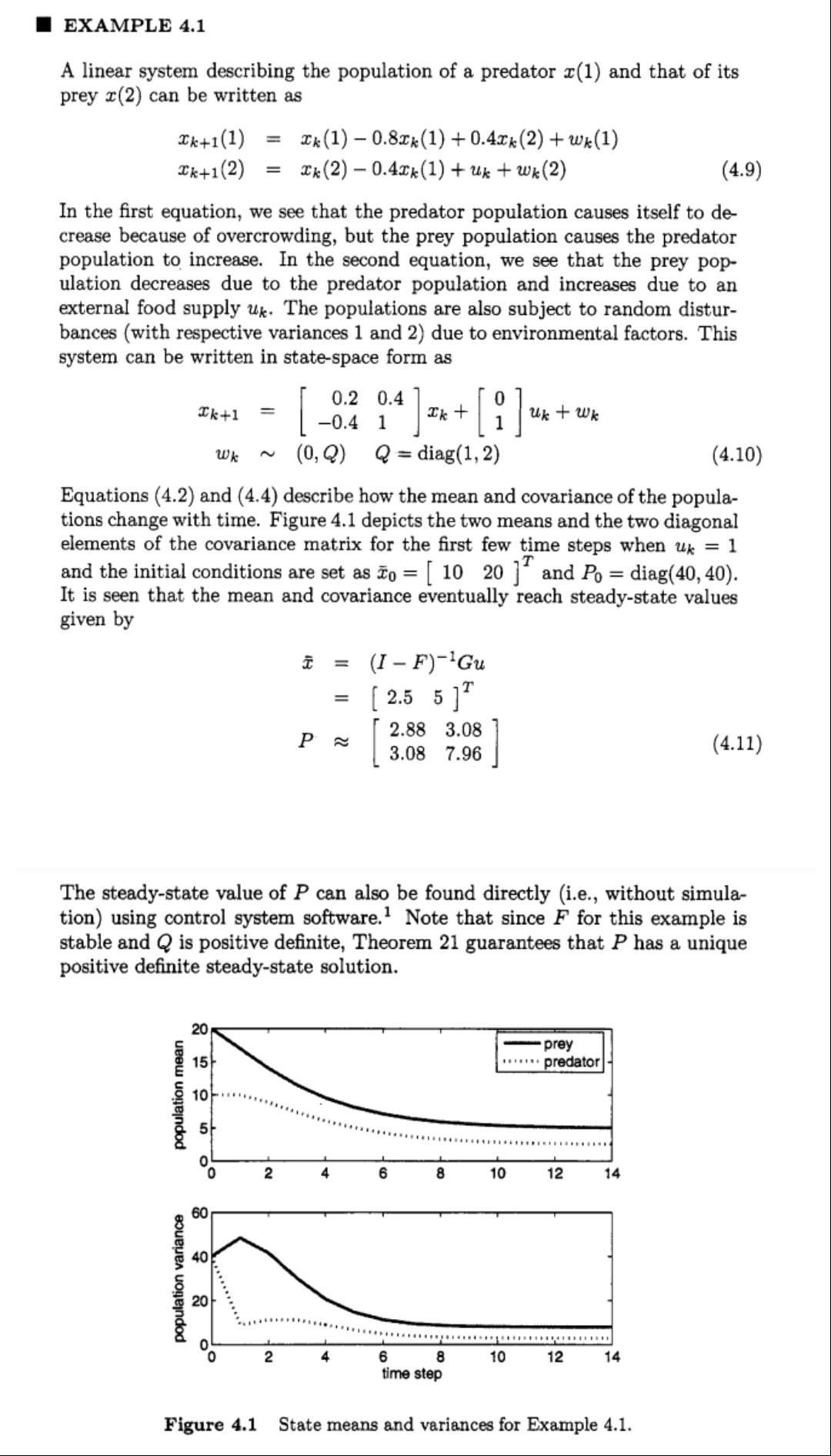
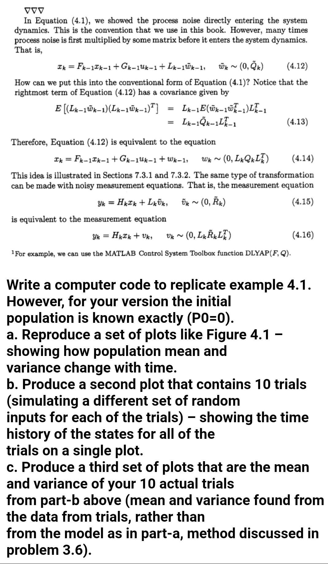
A linear system describing the population of a predator x(1) and that of its prey x(2) can be written as xk+1(1)=xk(1)0.8xk(1)+0.4xk(2)+wk(1)xk+1(2)=xk(2)0.4xk(1)+uk+wk(2) In the first equation, we see that the predator population causes itself to decrease because of overcrowding, but the prey population causes the predator population to increase. In the second equation, we see that the prey population decreases due to the predator population and increases due to an external food supply uk. The populations are also subject to random disturbances (with respective variances 1 and 2) due to environmental factors. This system can be written in state-space form as xk+1wk=[0.20.40.41]xk+[01]uk+wk(0,Q)Q=diag(1,2) Equations (4.2) and (4.4) describe how the mean and covariance of the populations change with time. Figure 4.1 depicts the two means and the two diagonal elements of the covariance matrix for the first few time steps when uk=1 and the initial conditions are set as x0=[1020]T and P0=diag(40,40). It is seen that the mean and covariance eventually reach steady-state values given by xP=(IF)1Gu=[2.55]T[2.883.083.087.96] The steady-state value of P can also be found directly (i.e., without simulation) using control system software. 1 Note that since F for this example is stable and Q is positive definite, Theorem 21 guarantees that P has a unique positive definite steady-state solution. Figure 4.1 State means and variances for Example 4.1. In Equation (4.1), we showed the process noise directly entering the system dynamics. This is the convention that we use in this book. However, many times process noise is first multiplied by some matrix before it enters the system dynamics. That is, xk=Fk1xk1+Gk1uk1+Lk1w~k1,w~k(0,Q~k) How can we put this into the conventional form of Equation (4.1)? Notice that the rightmost term of Equation (4.12) has a covariance given by E[(Lk1w~k1)(Lk1w~k1)T]=Lk1E(w~k1w~k1T)Lk1T=Lk1Q~k1Lk1T Therefore, Equation (4.12) is equivalent to the equation xk=Fk1xk1+Gk1uk1+wk1,wk(0,LkQkLkT)(4.14) This idea is illustrated in Sections 7.3.1 and 7.3.2. The same type of transformation can be made with noisy measurement equations. That is, the measurement equation yk=Hkxk+Lkv~k,v~k(0,R~k) is equivalent to the measurement equation yk=Hkxk+vk,vk(0,LkR~kLkT) 1 For example, we can use the MATLAB Control System Toolbox function DLYAP(F,Q). Write a computer code to replicate example 4.1. However, for your version the initial population is known exactly (PO=0). a. Reproduce a set of plots like Figure 4.1 showing how population mean and variance change with time. b. Produce a second plot that contains 10 trials (simulating a different set of random inputs for each of the trials) - showing the time history of the states for all of the trials on a single plot. c. Produce a third set of plots that are the mean and variance of your 10 actual trials from part-b above (mean and variance found fron the data from trials, rather than from the model as in part-a, method discussed in A linear system describing the population of a predator x(1) and that of its prey x(2) can be written as xk+1(1)=xk(1)0.8xk(1)+0.4xk(2)+wk(1)xk+1(2)=xk(2)0.4xk(1)+uk+wk(2) In the first equation, we see that the predator population causes itself to decrease because of overcrowding, but the prey population causes the predator population to increase. In the second equation, we see that the prey population decreases due to the predator population and increases due to an external food supply uk. The populations are also subject to random disturbances (with respective variances 1 and 2) due to environmental factors. This system can be written in state-space form as xk+1wk=[0.20.40.41]xk+[01]uk+wk(0,Q)Q=diag(1,2) Equations (4.2) and (4.4) describe how the mean and covariance of the populations change with time. Figure 4.1 depicts the two means and the two diagonal elements of the covariance matrix for the first few time steps when uk=1 and the initial conditions are set as x0=[1020]T and P0=diag(40,40). It is seen that the mean and covariance eventually reach steady-state values given by xP=(IF)1Gu=[2.55]T[2.883.083.087.96] The steady-state value of P can also be found directly (i.e., without simulation) using control system software. 1 Note that since F for this example is stable and Q is positive definite, Theorem 21 guarantees that P has a unique positive definite steady-state solution. Figure 4.1 State means and variances for Example 4.1. In Equation (4.1), we showed the process noise directly entering the system dynamics. This is the convention that we use in this book. However, many times process noise is first multiplied by some matrix before it enters the system dynamics. That is, xk=Fk1xk1+Gk1uk1+Lk1w~k1,w~k(0,Q~k) How can we put this into the conventional form of Equation (4.1)? Notice that the rightmost term of Equation (4.12) has a covariance given by E[(Lk1w~k1)(Lk1w~k1)T]=Lk1E(w~k1w~k1T)Lk1T=Lk1Q~k1Lk1T Therefore, Equation (4.12) is equivalent to the equation xk=Fk1xk1+Gk1uk1+wk1,wk(0,LkQkLkT)(4.14) This idea is illustrated in Sections 7.3.1 and 7.3.2. The same type of transformation can be made with noisy measurement equations. That is, the measurement equation yk=Hkxk+Lkv~k,v~k(0,R~k) is equivalent to the measurement equation yk=Hkxk+vk,vk(0,LkR~kLkT) 1 For example, we can use the MATLAB Control System Toolbox function DLYAP(F,Q). Write a computer code to replicate example 4.1. However, for your version the initial population is known exactly (PO=0). a. Reproduce a set of plots like Figure 4.1 showing how population mean and variance change with time. b. Produce a second plot that contains 10 trials (simulating a different set of random inputs for each of the trials) - showing the time history of the states for all of the trials on a single plot. c. Produce a third set of plots that are the mean and variance of your 10 actual trials from part-b above (mean and variance found fron the data from trials, rather than from the model as in part-a, method discussed in