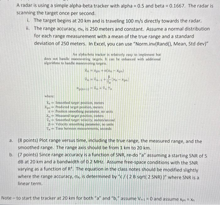
A radar is using a simple alpha-beta tracker with alpha =0.5 and beta =0.1667. The radar is scanning the target once per second. i. The target begins at 20km and is traveling 100m/s directly towards the radar. ii. The range accuracy, , is 250 meters and constant. Assume a normal distribution for each range measurement with a mean of the true range and a standard deviation of 250 meters. In Excel, you can use "Norm.inv(Rand(), Mean, Std dev)" An alpha-beta tracker is relatively easy to implement but dues not handle inatecuvering uagets. It can be cnhanced with additional algorithms to handle maneaverirg torgeis. xn=xna+(xnxnn)nvn+Ta(xnxpn)xp(n+1)/x0+vnTp where: xn= Smoothed target position, meters xpe= Predicted target position, meters a Position smoothing parameter no units xn= Measued target position. ficters yh= Smoothed target velocily, neters second . Velocity smoothing parameter, no units T. - Time between measurenents seconds. a. ( 8 points) Plot range versus time, including the true range, the measured range, and the smoothed range. The range axis should be from 1km to 20km. b. (7 points) Since range accuracy is a function of SNR, re-do "a" assuming a starting SNR of 5 dB at 20km and a bandwidth of 0.2MHz. Assume free-space conditions with the SNR varying as a function of R4. The equation in the class notes should be modified slightly where the range accuracy, R, is determined by " c/(2B sqrt( 2 SNR) )" where SNR is a linear term. Note - to start the tracker at 20km for both "a" and "b," assume Vn1=0 and assume xpn=xn A radar is using a simple alpha-beta tracker with alpha =0.5 and beta =0.1667. The radar is scanning the target once per second. i. The target begins at 20km and is traveling 100m/s directly towards the radar. ii. The range accuracy, , is 250 meters and constant. Assume a normal distribution for each range measurement with a mean of the true range and a standard deviation of 250 meters. In Excel, you can use "Norm.inv(Rand(), Mean, Std dev)" An alpha-beta tracker is relatively easy to implement but dues not handle inatecuvering uagets. It can be cnhanced with additional algorithms to handle maneaverirg torgeis. xn=xna+(xnxnn)nvn+Ta(xnxpn)xp(n+1)/x0+vnTp where: xn= Smoothed target position, meters xpe= Predicted target position, meters a Position smoothing parameter no units xn= Measued target position. ficters yh= Smoothed target velocily, neters second . Velocity smoothing parameter, no units T. - Time between measurenents seconds. a. ( 8 points) Plot range versus time, including the true range, the measured range, and the smoothed range. The range axis should be from 1km to 20km. b. (7 points) Since range accuracy is a function of SNR, re-do "a" assuming a starting SNR of 5 dB at 20km and a bandwidth of 0.2MHz. Assume free-space conditions with the SNR varying as a function of R4. The equation in the class notes should be modified slightly where the range accuracy, R, is determined by " c/(2B sqrt( 2 SNR) )" where SNR is a linear term. Note - to start the tracker at 20km for both "a" and "b," assume Vn1=0 and assume xpn=xn


