Also stat questions!

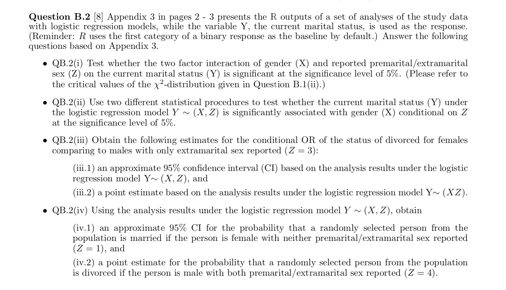
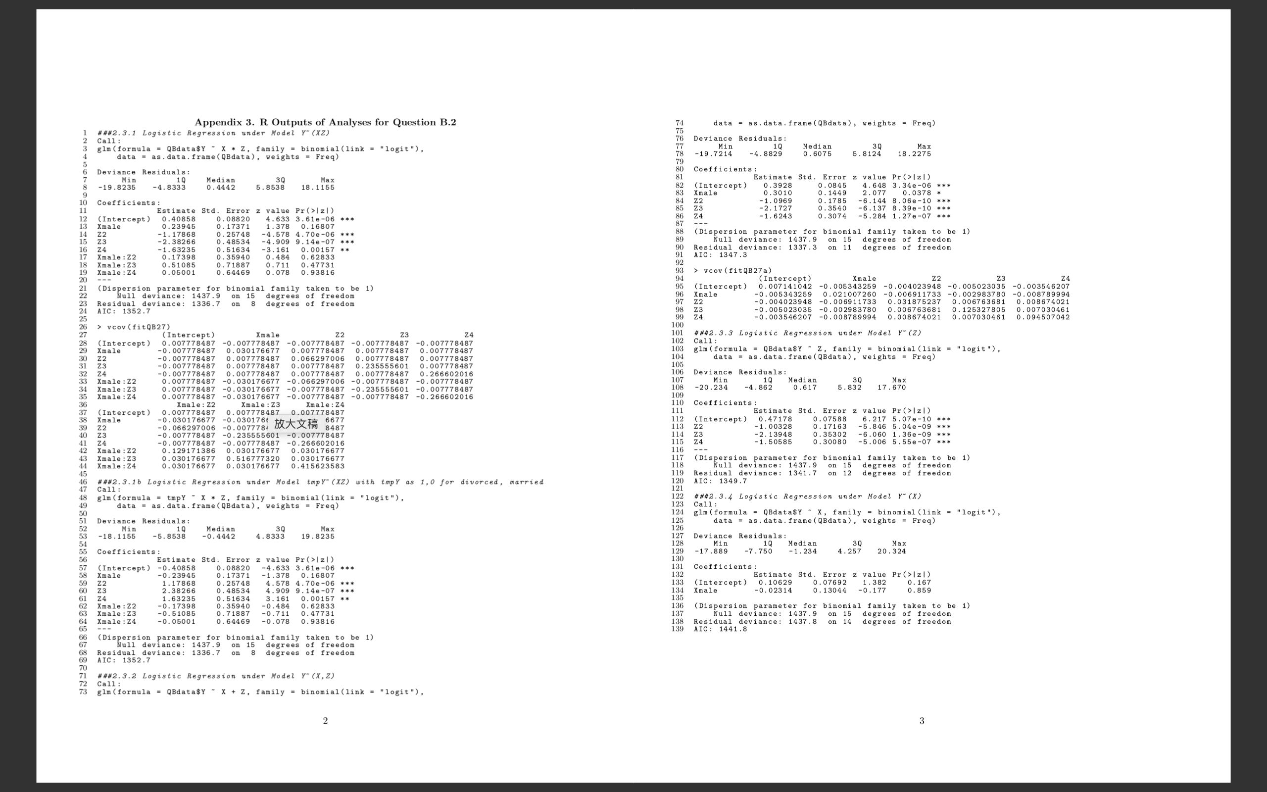
Question B.2 [8] Appendix 3 in pages 2 3 presents the R outputs of a set of analyses of the study data with logistic regression models, while the variable Y, the current marital status, is used as the response. (Reminder: R uses the rst category of a binary response as the baseline by default.) Answer the following questions based on Appendix 3. o QB.2(i) Test whether the two factor interaction of gender (X) and reported premarital/extramarital sex (Z) on the current marital status (Y) is signicant at the signicance level of 5%. (Please refer to the critical values of the X2distribution given in Question B.1(ii).) o QB.2(ii) Use two different statistical procedures to test whether the current marital status (Y) under the logistic regression model Y ~ (X, Z) is signicantly associated with gender (X) conditional on Z at the signicance level of 5%. o QB.2(iii) Obtain the following estimates for the conditional OR of the status of divorced for females comparing to males with only extramarital sex reported (Z = 3): (iii.1) an approximate 95% condence interval (CI) based on the analysis results under the logistic regression model Y~ (X, Z), and (iii.2) a point estimate based on the analysis results under the logistic regression model Y~ (X Z ) o QB.2(iv) Using the analysis results under the logistic regression model Y N (X, Z), obtain (iv.1) an approximate 95% CI for the probability that a randomly selected person from the population is married if the person is female with neither premarital/ extramarital sex reported (Z = 1), and (iv.2) a point estimate for the probability that a randomly selected person from the population is divorced if the person is male with both premarital / extramarital sex reported (Z = 4). Appendix 3. R Outputs of Analyses for Question B.2 Call : ###2.3.1 Logistic Regression under Model Y" (XZ) data = as . data . frame (QBdata), weights = Freq) glm (formula = QBdata$Y - X * Z, family = binomial(link = "logit"), Deviance Residuals: data = as . data . frame (QBdata), weights = Freq) Min 1Q Median 19 . 7214 -4. 8829 . 6075 5. 8124 18 . 2275 Deviance Residuals: Median Coefficients : -19 .8235 30 -4. 8333 0 . 4442 5. 8538 18 . 1155 Estimate Std. Error z value Pr (> |z ) (Intercept) 0. 3928 0 . 0845 Xmale 4. 648 3. 34e-06 * * Coefficients : 0 . 3010 0 . 1449 2 . 077 Z2 Estimate Std. Error z value Pr (>|z1 ) -1. 0969 0 . 1785 (Intercept ) 0. 40858 Z3 0 . 08820 -2. 1727 0 . 3540 -6. 144 8. 06e-10 * * * -6. 137 8. 39e-10 * * * Amale 0.23945 1:378 $3 3. 61e-06 ** * Z4 0. 16807 -1. 6243 0 . 3074 -5. 284 1. 27e-07 ** * Z2 15 -1. 17868 0 . 25748 Z3 -2. 38266 0 . 48534 -4.578 4.70e-06 * (Dispersion parameter for binomial family taken to be 1) 74 9 9. 14e-07 1 deviance: 1437.9 on 15 degrees of freedom 17 24 -1. 63235 0. 51634 -3. 161 0. 00157 * * Xmale : 22 0. 17398 0 . 35940 0. 484 0. 62833 90 Residual deviance: 1337.3 degrees of freedom 19 Xmale : Z3 0 . 51085 0 . 718 87 AIC : 1347.3 Xmale : 24 0 . 05001 20 0: 64469 0 . 711 0 . 078 . 93816 vcov (fitQB27a) (Dispersion parameter for binomial family taken to be 1) 8988288 (intercept) Xmale 22 Null deviance: 1437 .9 on 15 degrees of freedom (Intercept ) 0 . 007141042 Z2 -0. 005343259 -0.004023948 23 idual deviance: 1336.7 on 8 degrees of freedom Amale -0 . 005343259 -0 . 005023035 -0 . 003546207 AIC : 1352.7 Z2 -0 . 004023948 -0 006911733 31875237 -0. 002983780 -0. 008789994 74 -0 . 005023035 -0 . 002983780 0 . 006763681 99 0 . 006763681 0 . 125327805 0 . 007030461 > vcov (fitQB27) - 0 . 003546207 -0 . 008789994 0. 008674021 0 . 007030461 0 . 094507042 (Intercept) Xmale Z2 (Intercept) 0. 007778487 -0. 007778487 23 101 ###2.3.3 Logistic Regression under Model Y" (Z) Xmale -0. 007778487 -0. 007778487 24 -0. 007778487 0. 030176677 0. 007778487 -0 . 00777 0. 007778487 -0 . 007778487 102 Call : 0 . 007778487 103 glm (formula = QBdata$Y ~ Z, family = binomial (link = "logit"), Z3 -0. 007778487 0. 007778487 0. 066297006 32 74 778487 0 . 007778487 0. 007778487 0. 007778487 104 data = as . data . frame (QBdata) , weights = Freq) 24 -0 . 007778487 0. 007778487 35655601 0 . 007778487 105 33 0. 007778487 Xmale : Z2 0. 007778487 0. 007778487 0.266602016 34 0 . 030176677 -0.066297006 - 0 . 007778487 -0 . 007778487 -0. 007778487 Deviance Residuals Xmale : 23 -0. 030176677 -0.007778487 -0 .235555601 Min Median Xmale : Z4 0 . 007778487 -0. 030176677 -0. 007778487 -0. 007778487 . 007778487 -0 . 266602016 108 -20 .234 4. 862 0 . 617 5 . 832 Max 17 . 670 36 Xmale : Z2 Xmale : Z3 37 Xmale : Z4 1 10 (Intercept ) 0 . 007778487 Coefficients : Xmale 39 -0. 030176677 0. 007778487 0.007778487 -0. 0301761 -0 . 066297006 17784 XXXT $677 112 Estimate Std. Error z value Pr(>Izl) (Intercept) 0 . 47178 0 . 07588 40 23 -0. 007778487 -0 . 235555601 -0.007778487 113 Z2 1 . 00328 0 . 17163 7.4 -0.266602016 Z3 -2. 13948 6 5. 04e-09 -0. 007778487 -0. 007778487 0. 129171386 0 . 030176677 115 24 -1: 50585 0 . 35302 -8:060 1.36e-09 * Xmale : 22 0 . 30080 -5.006 5. 55e-07 * * * 44 Kmale : Z3 0 . 030176677 0 516777320 0. 030176677 0 030176677 116 Xmale : 24 . 030176677 0 . 030176677 0. 415623583 117 45 (Dispersion parameter for binomial family taken to be 1) 1 19 Null deviance: 1437 .9 on 15 degrees of freedom Call : 46 # ##2.3.1b Logistic Regression under Model tmpY" (XZ) with tmpY as 1,0 for divorced, married Residual deviance: 1341.7 on 12 AIC : 1349.7 degrees of freedom glm (formula = tmpY - X * Z, family = binomial (link = "logit"), 86 60 data = as . data . frame (QBdata) , weights = Freq) 123 122 # ##2.3.4 Logistic Regression under Model Y" (X) Deviance Residuals: 125 glm (formula = QBdata$Y ~ X, family = binomial (link = "logit"), data = as . data . frame (QBdata), weights = Freq) -18 . 1155 -5. 8538 Median -0. 4442 4. 8333 19 . 8235 126 Coefficients : 128 Deviance Residuals : 129 Min Median 3W Estimate Std. Error z value Pr (>|z1 ) 130 17 .889 -7 . 750 -1. 234 4 . 257 Max 20 . 324 (Intercept ) -0. 40858 0 . 08820 Amale -4.633 3 59 -0. 23945 -1.378 0. 16807 Coefficients : Estimate Std. Error z value Pr(> |zl) 60 22 1. 17868 0 . 25748 4. 578 4.70e-06 2.38266 0 . 48534 4. 909 9. 14e-07 (Intercept ) 0.10629 1. 63235 0. 51634 0. 00157 * * Xmale 0 . 07692 0 . 167 135 -0 . 02314 0 . 13044 -0 . 177 62 0 . 859 -0. 17398 63 Xmale : 22 0 . 35940 64 Amale : 23 -0. 51085 0 . 71887 -0. 484 0. 62833 -0.711 0. 47731 (Dispersion parameter for binomial family taken to be 1) 65 Xmale : 24 -0. 05001 0. 64469 -0. 078 0. 93816 137 138 Null deviance: 1437.9 on 15 degrees of freedom Residual deviance: 1437.8 on 14 degrees of freedom 66 139 (Dispersion parameter for binomial family taken to be 1) AIC: 1441 .8 Null deviance: 1437 .9 on 15 degrees of freedom 69 Residual deviance: 1336.7 on IC: 1352.7 8 degrees of freedom 70 72 Call : # ##2. 3.2 Logistic Regression under Model Y" (X, Z) 73 glm (formula = QBdata$Y ~ X + Z, family = binomial(link = "logit")