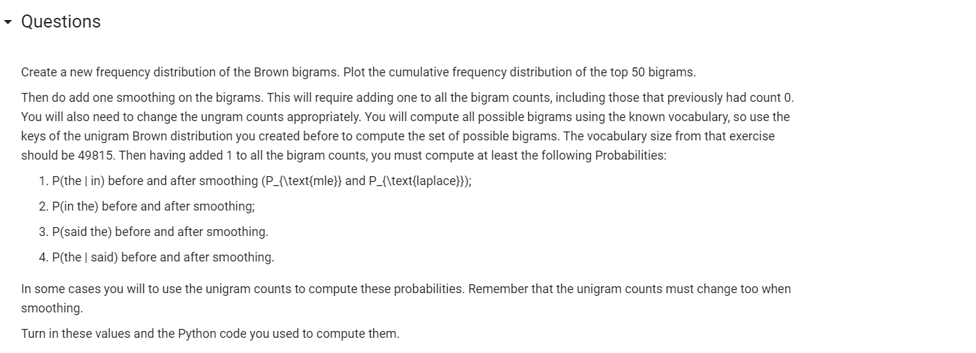
ANSWER FROM PREVIOUS QUESTION:  import nltk from nltk.corpus import brown dct = dict() for word in brown.words(): temp = dct.get(word,0) dct[word]=temp+1 a = list(dct.items()) a.sort(reverse=True,key=lambda x:x[1]) total = len(brown.words()) prop = 0 for i in range(20): prop+=a[i][1] print(f"{(prop/total):.2f}")

Questions Create a new frequency distribution of the Brown bigrams. Plot the cumulative frequency distribution of the top 50 bigrams. Then do add one smoothing on the bigrams. This will require adding one to all the bigram counts, including those that previously had count 0. You will also need to change the ungram counts appropriately. You will compute all possible bigrams using the known vocabulary, so use the keys of the unigram Brown distribution you created before to compute the set of possible bigrams. The vocabulary size from that exercise should be 49815. Then having added 1 to all the bigram counts, you must compute at least the following Probabilities: 1. P(the | in) before and after smoothing (P_{\text{mle}} and P_{\text{laplace}}); 2. P(in the) before and after smoothing; 3. P(said the) before and after smoothing. 4. P(the said) before and after smoothing. In some cases you will to use the unigram counts to compute these probabilities. Remember that the unigram counts must change too when smoothing. Turn in these values and the Python code you used to compute them. Questions Create a new frequency distribution of the Brown bigrams. Plot the cumulative frequency distribution of the top 50 bigrams. Then do add one smoothing on the bigrams. This will require adding one to all the bigram counts, including those that previously had count 0. You will also need to change the ungram counts appropriately. You will compute all possible bigrams using the known vocabulary, so use the keys of the unigram Brown distribution you created before to compute the set of possible bigrams. The vocabulary size from that exercise should be 49815. Then having added 1 to all the bigram counts, you must compute at least the following Probabilities: 1. P(the | in) before and after smoothing (P_{\text{mle}} and P_{\text{laplace}}); 2. P(in the) before and after smoothing; 3. P(said the) before and after smoothing. 4. P(the said) before and after smoothing. In some cases you will to use the unigram counts to compute these probabilities. Remember that the unigram counts must change too when smoothing. Turn in these values and the Python code you used to compute them