Answered step by step
Verified Expert Solution
Question
1 Approved Answer
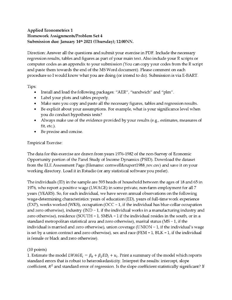
Applied Econometrics 1 Homework Assignments/Problem Set 4 Submission due: January 144 2021 (Thursday); 12:00NN. Direction: Answer all the questions and submit your exercise in PDF.


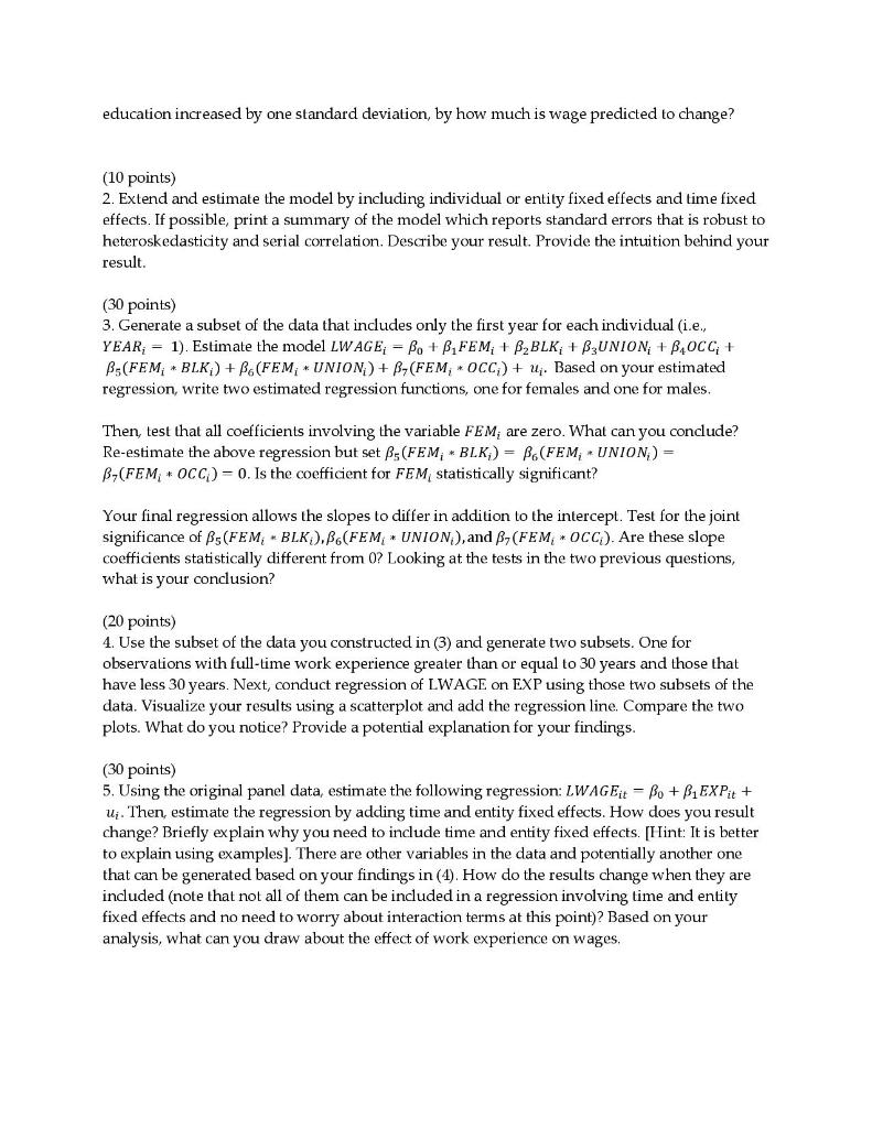
Applied Econometrics 1 Homework Assignments/Problem Set 4 Submission due: January 144 2021 (Thursday); 12:00NN. Direction: Answer all the questions and submit your exercise in PDF. Include the necessary regression results, tables and figures as part of your main text. Also include your R scripts or computer codes as an appendix to your submission (You can copy your codes from the script and paste them towards the end of the MS Word document). Please comment on each procedure so I would know what you are doing (or intend to do). Submission is via E-BART. Tips: . Install and load the following packages: "AER", "sandwich" and "plm". Label your plots and tables properly. Make sure you copy and paste all the necessary figures, tables and regression results. Be explicit about your assumptions. For example, what is your significance level when you do conduct hypothesis tests? Always make use of the evidence provided by your results (e.g., estimates, measures of fit, etc.). Be precise and concise. . . Empirical Exercise: The data for this exercise are drawn from years 1976-1982 of the non-Survey of Economic Opportunity portion of the Panel Study of Income Dynamics (PSID). Download the dataset from the ELE Assessment Page (filename: cornwell&rupert1988_rev.csv) and save it on your working directory. Load it in Rstudio (or any statistical software you prefer). The individuals (ID) in the sample are 595 heads of household between the ages of 18 and 65 in 1976, who report a positive wage (LWAGE) in some private, non-farm employment for all 7 years (YEARS). So, for each individual, we have seven annual observations on the following wage-determining characteristics: years of education (ED), years of full-time work experience (EXP), weeks worked (WKS), occupation (OCC = 1, if the individual has blue-collar occupation and zero otherwise), industry (IND-1, if the individual works in a manufacturing industry and zero otherwise), residence (SOUTH = 1, SMSA = 1 if the individual resides in the south, or in a standard metropolitan statistical area and zero otherwise), marital status (MS-1, if the individual is married and zero otherwise), union coverage (UNION = 1, if the individual's wage is set by a union contract and zero otherwise), sex and race (FEM = 1, BLK = 1, if the individual is female or black and zero otherwise). (10 points) 1. Estimate the model LWAGE; = Bo + B.ED; + ui. Print a summary of the model which reports standard errors that is robust to heteroskedasticity. Interpret the results: intercept, slope coefficient, R2 and standard error of regression. Is the slope coefficient statistically significant? If education increased by one standard deviation, by how much is wage predicted to change? (10 points) 2. Extend and estimate the model by including individual or entity fixed effects and time fixed effects. If possible, print a summary of the model which reports standard errors that is robust to heteroskedasticity and serial correlation. Describe your result. Provide the intuition behind your result (30 points) 3. Generate a subset of the data that includes only the first year for each individual (i.e., YEAR; = 1). Estimate the model LWAGE; - Be + B FEM + B2BLK; + BUNION; + BLOCC; + B:(FEM* BLK) + B.(FEM; * UNION) + B-(FEM, * OCC;) + up. Based on your estimated regression, write two estimated regression functions, one for females and one for males. Then, test that all coefficients involving the variable FEM; are zero. What can you conclude? Re-estimate the above regression but set B-(FEM; * BLK;) = B.(FEM; * UNION) = B(FEM * OCC) = 0. Is the coefficient for FEM statistically significant? Your final regression allows the slopes to differ in addition to the intercept. Test for the joint significance of Bs(FEM-BLK).B.(FEM * UNION.), and B-(FEM, * OCC). Are these slope coefficients statistically different from 0? Looking at the tests in the two previous questions, what is your conclusion? (20 points) 4. Use the subset of the data you constructed in (3) and generate two subsets. One for observations with full-time work experience greater than or equal to 30 years and those that have less 30 years. Next, conduct regression of LWAGE on EXP using those two subsets of the data. Visualize your results using a scatterplot and add the regression line. Compare the two plots. What do you notice Provide a potential explanation for your findings. (30 points) 5. Using the original panel data, estimate the following regression: LWAGEit = Bo + B, EX Pit + u Then, estimate the regression by adding time and entity fixed effects. How does you result change? Briefly explain why you need to include time and entity fixed effects. [Hint: It is better to explain using examples). There are other variables in the data and potentially another one that can be generated based on your findings in (4). How do the results change when they are included (note that not all of them can be included in a regression involving time and entity fixed effects and no need to worry about interaction terms at this point)? Based on your analysis, what can you draw about the effect of work experience on wages, Applied Econometrics 1 Homework Assignments/Problem Set 4 Submission due: January 144 2021 (Thursday); 12:00NN. Direction: Answer all the questions and submit your exercise in PDF. Include the necessary regression results, tables and figures as part of your main text. Also include your R scripts or computer codes as an appendix to your submission (You can copy your codes from the script and paste them towards the end of the MS Word document). Please comment on each procedure so I would know what you are doing (or intend to do). Submission is via E-BART. Tips: . Install and load the following packages: "AER", "sandwich" and "plm". Label your plots and tables properly. Make sure you copy and paste all the necessary figures, tables and regression results. Be explicit about your assumptions. For example, what is your significance level when you do conduct hypothesis tests? Always make use of the evidence provided by your results (e.g., estimates, measures of fit, etc.). Be precise and concise. . . Empirical Exercise: The data for this exercise are drawn from years 1976-1982 of the non-Survey of Economic Opportunity portion of the Panel Study of Income Dynamics (PSID). Download the dataset from the ELE Assessment Page (filename: cornwell&rupert1988_rev.csv) and save it on your working directory. Load it in Rstudio (or any statistical software you prefer). The individuals (ID) in the sample are 595 heads of household between the ages of 18 and 65 in 1976, who report a positive wage (LWAGE) in some private, non-farm employment for all 7 years (YEARS). So, for each individual, we have seven annual observations on the following wage-determining characteristics: years of education (ED), years of full-time work experience (EXP), weeks worked (WKS), occupation (OCC = 1, if the individual has blue-collar occupation and zero otherwise), industry (IND-1, if the individual works in a manufacturing industry and zero otherwise), residence (SOUTH = 1, SMSA = 1 if the individual resides in the south, or in a standard metropolitan statistical area and zero otherwise), marital status (MS-1, if the individual is married and zero otherwise), union coverage (UNION = 1, if the individual's wage is set by a union contract and zero otherwise), sex and race (FEM = 1, BLK = 1, if the individual is female or black and zero otherwise). (10 points) 1. Estimate the model LWAGE; = Bo + B.ED; + ui. Print a summary of the model which reports standard errors that is robust to heteroskedasticity. Interpret the results: intercept, slope coefficient, R2 and standard error of regression. Is the slope coefficient statistically significant? If education increased by one standard deviation, by how much is wage predicted to change? (10 points) 2. Extend and estimate the model by including individual or entity fixed effects and time fixed effects. If possible, print a summary of the model which reports standard errors that is robust to heteroskedasticity and serial correlation. Describe your result. Provide the intuition behind your result (30 points) 3. Generate a subset of the data that includes only the first year for each individual (i.e., YEAR; = 1). Estimate the model LWAGE; - Be + B FEM + B2BLK; + BUNION; + BLOCC; + B:(FEM* BLK) + B.(FEM; * UNION) + B-(FEM, * OCC;) + up. Based on your estimated regression, write two estimated regression functions, one for females and one for males. Then, test that all coefficients involving the variable FEM; are zero. What can you conclude? Re-estimate the above regression but set B-(FEM; * BLK;) = B.(FEM; * UNION) = B(FEM * OCC) = 0. Is the coefficient for FEM statistically significant? Your final regression allows the slopes to differ in addition to the intercept. Test for the joint significance of Bs(FEM-BLK).B.(FEM * UNION.), and B-(FEM, * OCC). Are these slope coefficients statistically different from 0? Looking at the tests in the two previous questions, what is your conclusion? (20 points) 4. Use the subset of the data you constructed in (3) and generate two subsets. One for observations with full-time work experience greater than or equal to 30 years and those that have less 30 years. Next, conduct regression of LWAGE on EXP using those two subsets of the data. Visualize your results using a scatterplot and add the regression line. Compare the two plots. What do you notice Provide a potential explanation for your findings. (30 points) 5. Using the original panel data, estimate the following regression: LWAGEit = Bo + B, EX Pit + u Then, estimate the regression by adding time and entity fixed effects. How does you result change? Briefly explain why you need to include time and entity fixed effects. [Hint: It is better to explain using examples). There are other variables in the data and potentially another one that can be generated based on your findings in (4). How do the results change when they are included (note that not all of them can be included in a regression involving time and entity fixed effects and no need to worry about interaction terms at this point)? Based on your analysis, what can you draw about the effect of work experience on wages
Step by Step Solution
There are 3 Steps involved in it
Step: 1

Get Instant Access to Expert-Tailored Solutions
See step-by-step solutions with expert insights and AI powered tools for academic success
Step: 2

Step: 3

Ace Your Homework with AI
Get the answers you need in no time with our AI-driven, step-by-step assistance
Get Started


