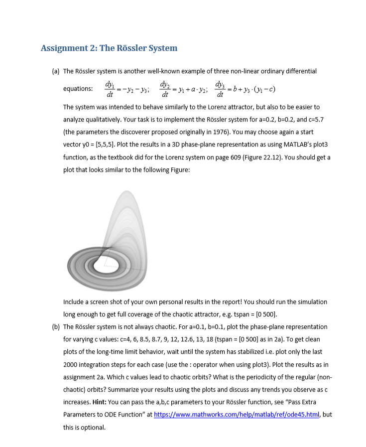
Assignment 2: The Rssler System (a) The Rssler system is another well-known example of three non-linear ordinary differential dvi dt equations:2-iab+(-c) The system was intended to behave similarly to the Lorenz attractor, but also to be easier to analyze qualitatively. Your task is to implement the Rssler system for a-0.2, b-0.2, and c 5.7 (the parameters the discoverer proposed originally in 1976). You may choose again a start vector yo = [5,5,5]. Plot the results in a 3D phase-plane representation as using MATLAB's plot3 function, as the textbook did for the Lorenz system on page 609 (Figure 22.12). You should get a plot that looks similar to the following Figure dt dt Include a screen shot of your own personal results in the report! You should run the simulation long enough to get full coverage of the chaotic attractor, e.g. tspan [0 500]. (b) The Rssler system is not always chaotic. For a-0.1, b-0.1, plot the phase-planerepresentation for varying c values: c-4, 6, 8.5, 8.7, 9, 12, 12.6, 13, 18 (tspan [0 500] as in 2a). To get clean plots of the long-time limit behavior, wait until the system has stabilized i.e. plot only the last 2000 integration steps for each case (use the: operator when using plot3). Plot the results as in assignment 2a. Which c values lead to chaotic orbits? What is the periodicity of the regular (non chaotic) orbits? Summarize your results using the plots and discuss any trends you observe as c increases. Hint: You can pass the a,b,c parametes to your Rssler function, see "Pass Extra Parameters to ODE Function" at https://www.mathworks.com/help/matlab/ref/ode45.html, but this is optional. Assignment 2: The Rssler System (a) The Rssler system is another well-known example of three non-linear ordinary differential dvi dt equations:2-iab+(-c) The system was intended to behave similarly to the Lorenz attractor, but also to be easier to analyze qualitatively. Your task is to implement the Rssler system for a-0.2, b-0.2, and c 5.7 (the parameters the discoverer proposed originally in 1976). You may choose again a start vector yo = [5,5,5]. Plot the results in a 3D phase-plane representation as using MATLAB's plot3 function, as the textbook did for the Lorenz system on page 609 (Figure 22.12). You should get a plot that looks similar to the following Figure dt dt Include a screen shot of your own personal results in the report! You should run the simulation long enough to get full coverage of the chaotic attractor, e.g. tspan [0 500]. (b) The Rssler system is not always chaotic. For a-0.1, b-0.1, plot the phase-planerepresentation for varying c values: c-4, 6, 8.5, 8.7, 9, 12, 12.6, 13, 18 (tspan [0 500] as in 2a). To get clean plots of the long-time limit behavior, wait until the system has stabilized i.e. plot only the last 2000 integration steps for each case (use the: operator when using plot3). Plot the results as in assignment 2a. Which c values lead to chaotic orbits? What is the periodicity of the regular (non chaotic) orbits? Summarize your results using the plots and discuss any trends you observe as c increases. Hint: You can pass the a,b,c parametes to your Rssler function, see "Pass Extra Parameters to ODE Function" at https://www.mathworks.com/help/matlab/ref/ode45.html, but this is optional