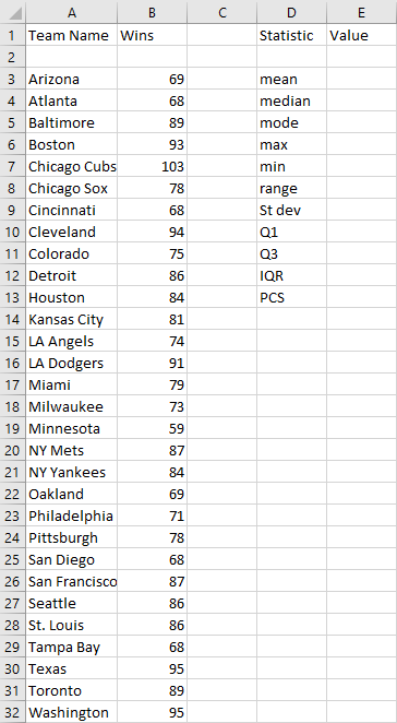
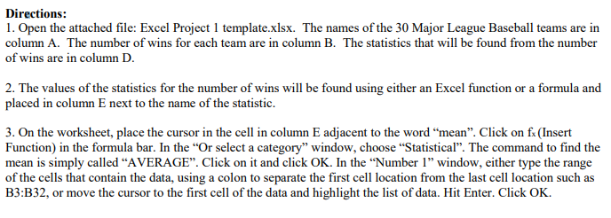
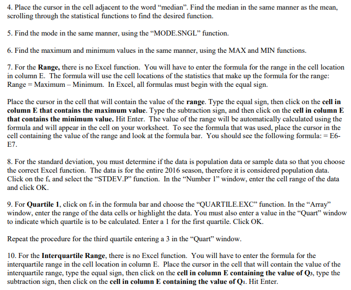
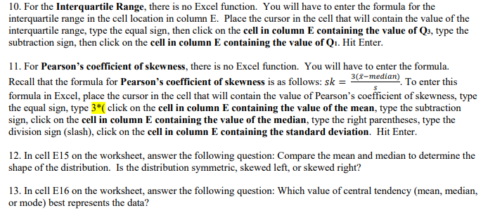
B C D A 1 Team Name Wins 2 3 Arizona E Statistic Value 69 4 Atlanta 68 5 Baltimore 89 mean median mode 6 Boston 93 max 7 Chicago Cubs 103 min 8 Chicago Sox 78 9 Cincinnati 68 range St dev 10 Cleveland 94 Q1 11 Colorado 75 Q3 12 Detroit 86 IQR 13 Houston 84 PCS 14 Kansas City 81 15 LA Angels 74 16 LA Dodgers 91 17 Miami 79 18 Milwaukee 73 19 Minnesota 59 20 NY Mets 87 21 NY Yankees 84 22 Oakland 69 23 Philadelphia 71 24 Pittsburgh 78 25 San Diego 68 26 San Francisco 87 27 Seattle 86 28 St. Louis 86 29 Tampa Bay 68 30 Texas 95 31 Toronto 89 32 Washington 95 Directions: 1. Open the attached file: Excel Project 1 template.xlsx. The names of the 30 Major League Baseball teams are in column A. The number of wins for each team are in column B. The statistics that will be found from the number of wins are in column D. 2. The values of the statistics for the number of wins will be found using either an Excel function or a formula and placed in column E next to the name of the statistic. 3. On the worksheet, place the cursor in the cell in column E adjacent to the word "mean". Click on fx (Insert Function) in the formula bar. In the "Or select a category" window, choose "Statistical". The command to find the mean is simply called "AVERAGE". Click on it and click OK. In the "Number 1" window, either type the range of the cells that contain the data, using a colon to separate the first cell location from the last cell location such as B3:B32, or move the cursor to the first cell of the data and highlight the list of data. Hit Enter. Click OK. 4. Place the cursor in the cell adjacent to the word "median". Find the median in the same manner as the mean, scrolling through the statistical functions to find the desired function. 5. Find the mode in the same manner, using the "MODE.SNGL" function. 6. Find the maximum and minimum values in the same manner, using the MAX and MIN functions. 7. For the Range, there is no Excel function. You will have to enter the formula for the range in the cell location in column E. The formula will use the cell locations of the statistics that make up the formula for the range: Range = Maximum - Minimum. In Excel, all formulas must begin with the equal sign. Place the cursor in the cell that will contain the value of the range. Type the equal sign, then click on the cell in column E that contains the maximum value. Type the subtraction sign, and then click on the cell in column E that contains the minimum value. Hit Enter. The value of the range will be automatically calculated using the formula and will appear in the cell on your worksheet. To see the formula that was used, place the cursor in the cell containing the value of the range and look at the formula bar. You should see the following formula: =E6- E7. 8. For the standard deviation, you must determine if the data is population data or sample data so that you choose the correct Excel function. The data is for the entire 2016 season, therefore it is considered population data. Click on the fx and select the "STDEV.P" function. In the "Number 1" window, enter the cell range of the data and click OK. 9. For Quartile 1, click on fx in the formula bar and choose the "QUARTILE.EXC" function. In the "Array" window, enter the range of the data cells or highlight the data. You must also enter a value in the "Quart" window to indicate which quartile is to be calculated. Enter a 1 for the first quartile. Click OK. Repeat the procedure for the third quartile entering a 3 in the "Quart" window. 10. For the Interquartile Range, there is no Excel function. You will have to enter the formula for the interquartile range in the cell location in column E. Place the cursor in the cell that will contain the value of the interquartile range, type the equal sign, then click on the cell in column E containing the value of Q3, type the subtraction sign, then click on the cell in column E containing the value of Qi. Hit Enter. 10. For the Interquartile Range, there is no Excel function. You will have to enter the formula for the interquartile range in the cell location in column E. Place the cursor in the cell that will contain the value of the interquartile range, type the equal sign, then click on the cell in column E containing the value of Q3, type the subtraction sign, then click on the cell in column E containing the value of Q1. Hit Enter. S 11. For Pearson's coefficient of skewness, there is no Excel function. You will have to enter the formula. 3(x-median) To enter this Recall that the formula for Pearson's coefficient of skewness is as follows: sk = formula in Excel, place the cursor in the cell that will contain the value of Pearson's coefficient of skewness, type the equal sign, type 3*( click on the cell in column E containing the value of the mean, type the subtraction sign, click on the cell in column E containing the value of the median, type the right parentheses, type the division sign (slash), click on the cell in column E containing the standard deviation. Hit Enter. 12. In cell E15 on the worksheet, answer the following question: Compare the mean and median to determine the shape of the distribution. Is the distribution symmetric, skewed left, or skewed right? 13. In cell E16 on the worksheet, answer the following question: Which value of central tendency (mean, median, or mode) best represents the data?