CA2_1.mat:

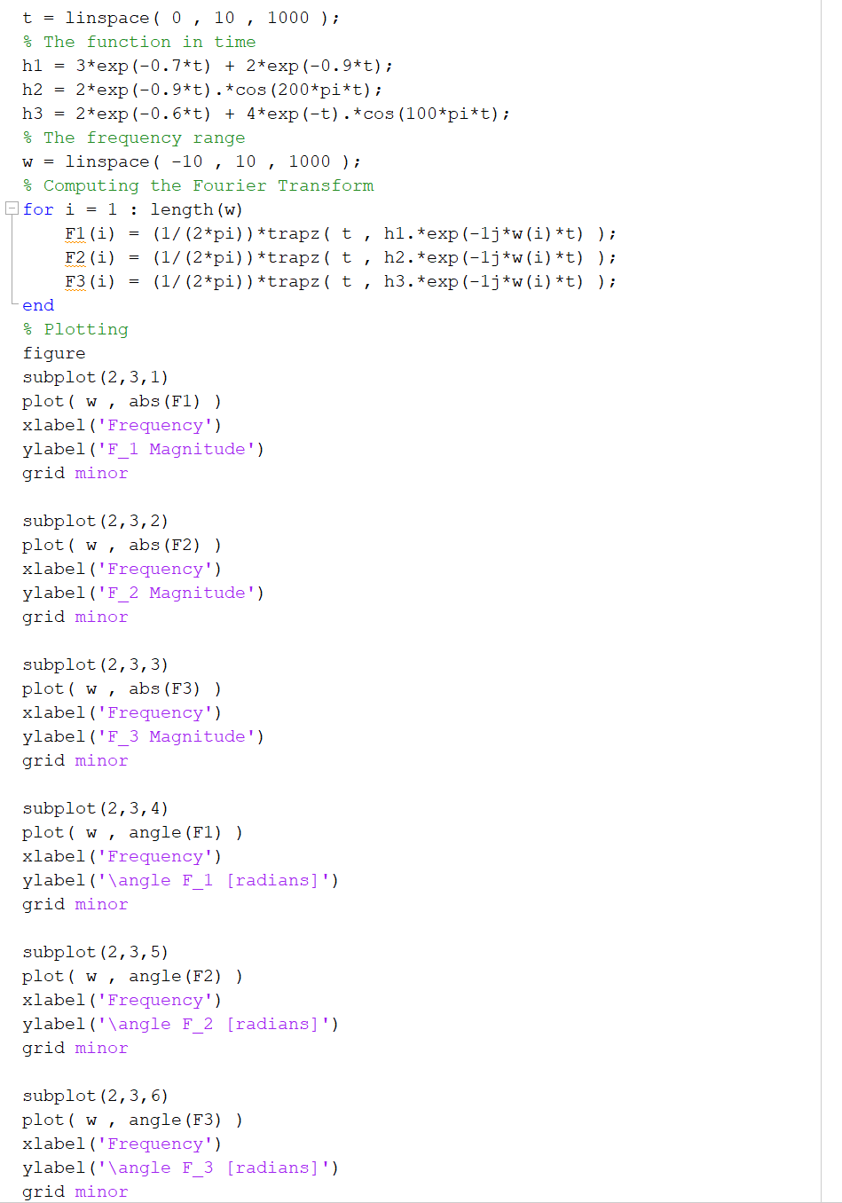
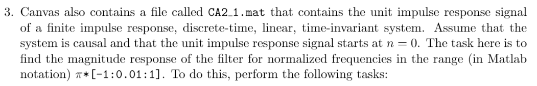
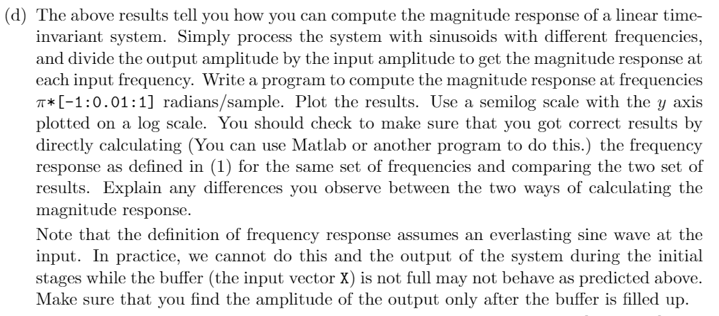
3. Canvas also contains a file called CA2_1.mat that contains the unit impulse response signal of a finite impulse response, discrete-time, linear, time-invariant system. Assume that the system is causal and that the unit impulse response signal starts at n = 0. The task here is to find the magnitude response of the filter for normalized frequencies in the range (in Matlab notation) **[-1:0.01:1]. To do this, perform the following tasks: (d) The above results tell you how you can compute the magnitude response of a linear time- invariant system. Simply process the system with sinusoids with different frequencies, and divide the output amplitude by the input amplitude to get the magnitude response at each input frequency. Write a program to compute the magnitude response at frequencies T*[-1:0.01:1] radians/sample. Plot the results. Use a semilog scale with the y axis plotted on a log scale. You should check to make sure that you got correct results by directly calculating (You can use Matlab or another program to do this.) the frequency response as defined in (1) for the same set of frequencies and comparing the two set of results. Explain any differences you observe between the two ways of calculating the magnitude response. Note that the definition of frequency response assumes an everlasting sine wave at the input. In practice, we cannot do this and the output of the system during the initial stages while the buffer (the input vector X) is not full may not behave as predicted above. Make sure that you find the amplitude of the output only after the buffer is filled up. t = linspace ( 0 , 10 , 1000); % The function in time hl = 3*exp(-0.7*t) + 2*exp(-0.9*t); h2 2*exp(-0.9*t).*cos (200*pi*t); h3 = 2*exp(-0.6*t) + 4*exp(-t).*cos (100*pi*t); % The frequency range w = linspace( -10 , 10 , 1000); % Computing the Fourier Transform for i = 1 : length (w) F1 (i) = (1/(2*pi))*trapz ( t, hl.*exp(-1j*w(i)*t) ); F2 (i) (1/(2*pi))*trapz( t, h2.*exp(-1j+w(i)*t) ); F3 (i) (1/(2*pi))*trapz ( t , h3.*exp(-1j*w(i)*t)); end % Plotting figure subplot (2,3,1) plot ( w, abs (F1) ) xlabel('Frequency') ylabel ('F_1 Magnitude') grid minor subplot (2,3,2) plot(w , abs (F2) ) xlabel('Frequency') ylabel('F_2 Magnitude') grid minor subplot (2,3,3) plot(w , abs (F3) ) xlabel('Frequency') ylabel ('F_3 Magnitude') grid minor subplot (2,3,4) plot(w, angle (F1) ) xlabel ('Frequency') ylabel('\angle F_1 [radians]') grid minor subplot (2,3,5) plot ( w, angle (F2)) xlabel ('Frequency') ylabel('\angle F_2 [radians]') grid minor subplot (2,3,6) plot( w, angle (F3) ) xlabel ('Frequency') ylabel('\angle F_3 [radians]') grid minor 3. Canvas also contains a file called CA2_1.mat that contains the unit impulse response signal of a finite impulse response, discrete-time, linear, time-invariant system. Assume that the system is causal and that the unit impulse response signal starts at n = 0. The task here is to find the magnitude response of the filter for normalized frequencies in the range (in Matlab notation) **[-1:0.01:1]. To do this, perform the following tasks: (d) The above results tell you how you can compute the magnitude response of a linear time- invariant system. Simply process the system with sinusoids with different frequencies, and divide the output amplitude by the input amplitude to get the magnitude response at each input frequency. Write a program to compute the magnitude response at frequencies T*[-1:0.01:1] radians/sample. Plot the results. Use a semilog scale with the y axis plotted on a log scale. You should check to make sure that you got correct results by directly calculating (You can use Matlab or another program to do this.) the frequency response as defined in (1) for the same set of frequencies and comparing the two set of results. Explain any differences you observe between the two ways of calculating the magnitude response. Note that the definition of frequency response assumes an everlasting sine wave at the input. In practice, we cannot do this and the output of the system during the initial stages while the buffer (the input vector X) is not full may not behave as predicted above. Make sure that you find the amplitude of the output only after the buffer is filled up. t = linspace ( 0 , 10 , 1000); % The function in time hl = 3*exp(-0.7*t) + 2*exp(-0.9*t); h2 2*exp(-0.9*t).*cos (200*pi*t); h3 = 2*exp(-0.6*t) + 4*exp(-t).*cos (100*pi*t); % The frequency range w = linspace( -10 , 10 , 1000); % Computing the Fourier Transform for i = 1 : length (w) F1 (i) = (1/(2*pi))*trapz ( t, hl.*exp(-1j*w(i)*t) ); F2 (i) (1/(2*pi))*trapz( t, h2.*exp(-1j+w(i)*t) ); F3 (i) (1/(2*pi))*trapz ( t , h3.*exp(-1j*w(i)*t)); end % Plotting figure subplot (2,3,1) plot ( w, abs (F1) ) xlabel('Frequency') ylabel ('F_1 Magnitude') grid minor subplot (2,3,2) plot(w , abs (F2) ) xlabel('Frequency') ylabel('F_2 Magnitude') grid minor subplot (2,3,3) plot(w , abs (F3) ) xlabel('Frequency') ylabel ('F_3 Magnitude') grid minor subplot (2,3,4) plot(w, angle (F1) ) xlabel ('Frequency') ylabel('\angle F_1 [radians]') grid minor subplot (2,3,5) plot ( w, angle (F2)) xlabel ('Frequency') ylabel('\angle F_2 [radians]') grid minor subplot (2,3,6) plot( w, angle (F3) ) xlabel ('Frequency') ylabel('\angle F_3 [radians]') grid minor