Can someone help me with question 2d) ONLY?

Can someone help me with question 2d) ONLY?

Can someone help me with question 2d) ONLY?

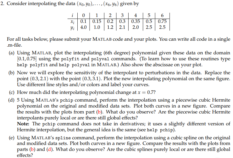
2. Consider interpolating the data (x0,yo), . . . , (x64%) given by Xi | 0.1 | 0.15 | 0.2 | 0.3 | 0.35 | 0.5 | 0.75 yi 4.0 1.0 1.22.12.02.52.5 For all tasks below, please submit your MATLAB code and your plots. You can write all code in a single (a) Using MATLAB, plot the interpolating (6th degree) polynomial given these data on the domain .m-file [0.1,0.75] using the polyfit and polyval commands. To learn how to use these routines type help polyfit and help polyval in MATLAB.) Also show the abscissae on your plot (b) Now we will explore the sensitivity of the interpolant to perturbations in the data. Replace the point (0.3,2.1) with the point (0.3,3.1). Plot the new interpolating polynomial on the same figure Use different line styles and/or colors and label your curves (c) How much did the interpolating polynomial change at x-0.7? (d) 5 Using MaTLAB's pchip command, perform the interpolation using a piecewise cubic Hermite polynomial on the original and modified data sets. Plot both curves in a new figure. Compare the results with the plots from part (b). What do you observe? Are the piecewise cubic Hermite interpolants purely local or are there still global effects? Note: The pchip command does not take in derivatives; it uses a slightly different version of Hermite interpolation, but the general idea is the same (see help pchip) (e) Using MATLAB's spline command, perform the interpolation using a cubic spline on the original and modified data sets. Plot both curves in a new figure. Compare the results with the plots from parts (b) and (d). What do you observe? Are the cubic splines purely local or are there still global effects? 2. Consider interpolating the data (x0,yo), . . . , (x64%) given by Xi | 0.1 | 0.15 | 0.2 | 0.3 | 0.35 | 0.5 | 0.75 yi 4.0 1.0 1.22.12.02.52.5 For all tasks below, please submit your MATLAB code and your plots. You can write all code in a single (a) Using MATLAB, plot the interpolating (6th degree) polynomial given these data on the domain .m-file [0.1,0.75] using the polyfit and polyval commands. To learn how to use these routines type help polyfit and help polyval in MATLAB.) Also show the abscissae on your plot (b) Now we will explore the sensitivity of the interpolant to perturbations in the data. Replace the point (0.3,2.1) with the point (0.3,3.1). Plot the new interpolating polynomial on the same figure Use different line styles and/or colors and label your curves (c) How much did the interpolating polynomial change at x-0.7? (d) 5 Using MaTLAB's pchip command, perform the interpolation using a piecewise cubic Hermite polynomial on the original and modified data sets. Plot both curves in a new figure. Compare the results with the plots from part (b). What do you observe? Are the piecewise cubic Hermite interpolants purely local or are there still global effects? Note: The pchip command does not take in derivatives; it uses a slightly different version of Hermite interpolation, but the general idea is the same (see help pchip) (e) Using MATLAB's spline command, perform the interpolation using a cubic spline on the original and modified data sets. Plot both curves in a new figure. Compare the results with the plots from parts (b) and (d). What do you observe? Are the cubic splines purely local or are there still global effects