Can someone please just help? Everything is there, Thanks.

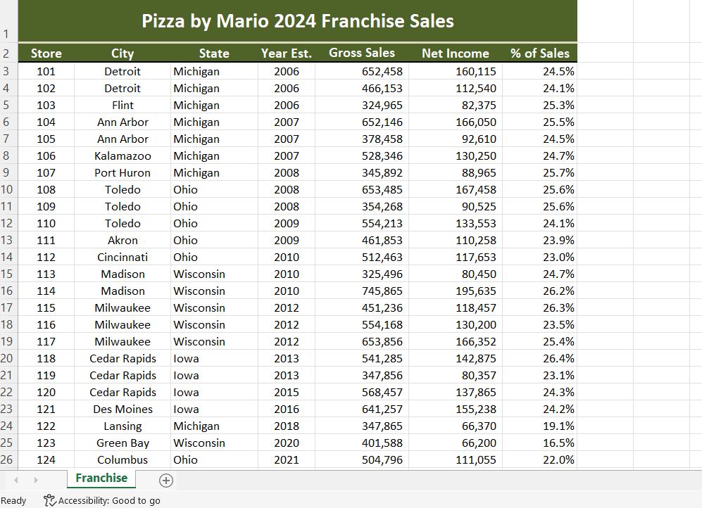
1-Yolanda Robertson, your manager at NuTrends Market Research, is continuing to work on the franchise expansion plan for the owners of Pizza by Mario. Yolanda has received a new workbook from the owners with profit information by store and would like you to summarize the data. Open the workbook PBMSales&Profits.xlsx, save it with the name 4-PBMRpt, and review the structure of the data. Yolanda has asked you to create a PivotTable that provides the average gross sales and average net income by city and state. You determine how to organize the layout of the report. Hint: You can add more than one numeric field to the Values list box. Apply formatting to improve the appearance of the report and make sure the report previews on one page in portrait orientation. Rename the worksheet containing the report PivotTable. Save 4-PBMRpt.xlsx.

2-Yolanda has asked you to create a chart that graphs the average net income data for the state of Michigan. Create a PivotChart in a new sheet named PivotChart and filter the chart appropriately to meet Yolandas request. You determine the appropriate chart style and elements to include in the chart. Yolanda will use this chart at an upcoming meeting with the franchise owners and wants it to be of professional quality. Preview the chart. Save the revised workbook with the name 4-PBMRpt-2 and then close the workbook.

3-Open 4-PBMRpt.xlsx and save it with the name 4-PBMRpt-3. Use the Help feature to find out how to modify a numeric field setting to show values as ranked numbers from largest to smallest. For example, instead of displaying the average value next to the city name, you will display the citys ranking as it compares with other cities in the same state. Ranking from largest to smallest means the highest value in the state is ranked as 1. Using the information you have learned in Help, change the display of the average sales to show the values ranked from largest to smallest using City as the base field. Remove the Net Income field from the PivotTable. Remove the Grand Total row at the bottom of the PivotTable. Hint: Use the Grand Totals button in the Layout group on the PivotTable Design tab. Make any other formatting changes to the report that you think will improve its appearance. Preview the PivotTable. Save 4-PBMRpt-3.xlsx.

4-Yolanda has asked you to do some comparison research on another pizza franchise. Use the internet to research the sales and net income of a pizza franchise you are familiar with. Create a new workbook that compares the total annual sales and net income values of the pizza franchise you researched with the Pizza By Mario information in 4-PBMRpt.xlsx. Provide the URL of the website from which you obtained the information about the competitor. Create a PivotTable that presents the comparison data. Save the workbook with the name 4-PizzaFranchiseComp. Preview the comparison data. Close 4-PizzaFranchiseComp.xlsx.

Pizza by Mario 2024 Franchise Sales Ready \& Accessibility: Good to go Ready 222 Accessibility: Good to go