Question: consider the econometric Lab#4, answer the questions. question: 7.7 ) Appendix: Econometric Lab #4 This lab is an exercise in specification: choosing the variables and


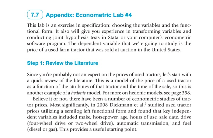
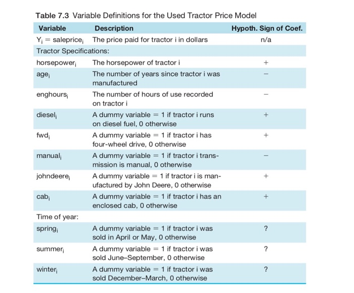
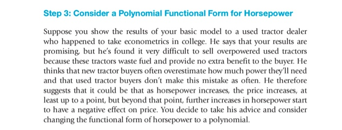
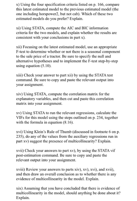
7.7 ) Appendix: Econometric Lab #4 This lab is an exercise in specification: choosing the variables and the func- tional form. It also will give you experience in transforming variables and conducting joint hypothesis tests in Stata or your computer's econometric software program. The dependent variable that we're going to study is the price of a used farm tractor that was sold at auction in the United States Step 1: Review the Literature Since you're probably not an expert on the prices of used tractors, let's start with a quick review of the literature. This is a model of the price of a used tractor as a function of the attributes of that tractor and the time of the sale, so this is another example of a hedonic model. For more on hedonic models, see page 358 Believe it or not, there have been a number of econometric studies of trac- tor prices. Most significantly, in 2008 Diekmann et al. studied used tractor prices utilizing a semilog left functional form and found that key indepen dent variables included make, horsepower, age, hours of use, sale date, drive (four-wheel drive or two-wheel drive), automatic transmission, and fuel (diesel or gas). This provides a useful starting point Table 7.3 Variable Definitions for the Used Tractor Price Model Variable Yi saleprice, The price paid for tractor i in dollars Tractor Specifications horsepower age Description Hypoth. Sign of Coef n/a The horsepower of tractor i enghours diesel fwd manual johndeere cab The number of years since tractor i was manufactured The number of hours of use recorded on tractor i A dummy variable 1 if tractor i runs on diesel fuel, 0 otherwise A dummy variable-1 if tractor i has four-wheel drive, O otherwise A dummy variable- 1 if tractor i trans- mission is manual, 0 otherwise A dummy variable-1 if tractor i is man- ufactured by John Deere, O otherwise A dummy variable1 if tractor i enclosed cab, 0 otherwise has an Time of year: springi A dummy variable- 1 if tractor i was sold in April or May, O otherwise A dummy variable1 if tractor i was sold June-September, O otherwise A dummy variable-1 if tractor i was sold December-March, 0 otherwise summe winter Step 2: Estimate the Basic Model As our basic model, let's estimate a variation of D more current dataset. Table 7.3 contains the definitions of the variables we'll need to attempt to replicate Diekmann's regression. The dependent variable is the price of a used farm tractor that was sold at auction in the United States between June 1, 2011 and May 31, 2012. The data0 are available on this text's website as dataset TRACTOR7. Table 7.3 also has the hypothesized expected sign of the coefficient of each variable, given the underlying theory. Now: n's model using a Step 3: Consider a Polynomial Functional Form for Horsepower Suppose you show the results of your basic model to a used tractor dealer who happened to take econometrics in college. He says that your results are promising, but he's found it very difficult to sell overpowered used tractors because these tractors waste fuel and provide no extra benefit to the buyer. He thinks that new tractor buyers often overestimate how much power they'll need and that used tractor buyers don't make this mistake as often. He therefore suggests that it could be that as horsepower increases, the price increases, at least up to a point, but beyond that point, further increases in horsepower start to have a negative effect on price. You decide to take his advice and consider changing the functional form of horsepower to a polynomial Step 4: Add a Potential Omitted Variable to Your Step 3 Model As ou're leaving the used tactor lot, you happen to notice that quite a few of the tractors have enclosed cabs. Since such a cab would come in handy in bad weather, you have a sudden sinking feeling that you might have an omitted variable! To test this, you find the data for cab (luckily also in TRACTOR7). Now: Step 5: Joint Hypothesis Testing Go back to the basic model of Step 2, and test at the 5-percent level the joint hypothesis that the time of year of the sale has no effect on the price of tractors: (Optional) Step 6: Consider a Slope Dummy That Interacts Diesel with Use It is well known that diesel engines tend to be more durable than gasoline That fact raises the q affects the value of a diesel tractor differently than for a gasoline tractor. Generate the variable you need to test this hypothesis, add this variable to the basic model of Step 2, estimate the revised slope dummy model, and test the appropriate slope dummy hypothesis at the 5-percent level. What is your -value? Can you reject the null hypothesis? x) Using the four specification criteria listed on p. 166, compare this latest estimated model to the previous estimated model (the one including horspower2, but not cab). Which of these two estimated models do you prefer? Explain. xi) Using STATA, compute the AIC and BIC information criteria for the two models, and explain whether the results are consistent with your conclusions in part x). xii) Focusing on the latest estimated model, use an appropriate F-test to determine whether or not there is a seasonal component to the sale price of a tractor. Be sure to specify the null and alternative hypotheses and to implement the F-test step-by-step using equation (5.10). xiii) Check your answer to part xii) by using the STATA test command. Be sure to copy and paste the relevant output into your assignment. xiv) Using STATA, compute the correlation matrix for the explanatory variables, and then cut and paste this correlation matrix into your assignment. xv) Using STATA to run the relevant regressions, calculate the VIFs for this model using the steps outlined on p. 234, together with the formula in equation (8.16. xvi) Using Klein's Rule of Thumb (discussed in footnote 6 on p 235), do any of the values from the auxiliary regressions run in part xv) suggest the presence of multicollinearity? Explain. xvii) Check your answers to part xv), by using the STATA vif post-estimation command. Be sure to copy and paste the relevant output into your assignment. x) Review your answers to parts xiv), xv), xvi), and xvii), and then draw an overall conclusion as to whether there is any evidence of multicollinearity in the model. Explain. xix) Assuming that you have concluded that there is evidence of multicollinearity in the model, should anything be done about it? Explain. 7.7 ) Appendix: Econometric Lab #4 This lab is an exercise in specification: choosing the variables and the func- tional form. It also will give you experience in transforming variables and conducting joint hypothesis tests in Stata or your computer's econometric software program. The dependent variable that we're going to study is the price of a used farm tractor that was sold at auction in the United States Step 1: Review the Literature Since you're probably not an expert on the prices of used tractors, let's start with a quick review of the literature. This is a model of the price of a used tractor as a function of the attributes of that tractor and the time of the sale, so this is another example of a hedonic model. For more on hedonic models, see page 358 Believe it or not, there have been a number of econometric studies of trac- tor prices. Most significantly, in 2008 Diekmann et al. studied used tractor prices utilizing a semilog left functional form and found that key indepen dent variables included make, horsepower, age, hours of use, sale date, drive (four-wheel drive or two-wheel drive), automatic transmission, and fuel (diesel or gas). This provides a useful starting point Table 7.3 Variable Definitions for the Used Tractor Price Model Variable Yi saleprice, The price paid for tractor i in dollars Tractor Specifications horsepower age Description Hypoth. Sign of Coef n/a The horsepower of tractor i enghours diesel fwd manual johndeere cab The number of years since tractor i was manufactured The number of hours of use recorded on tractor i A dummy variable 1 if tractor i runs on diesel fuel, 0 otherwise A dummy variable-1 if tractor i has four-wheel drive, O otherwise A dummy variable- 1 if tractor i trans- mission is manual, 0 otherwise A dummy variable-1 if tractor i is man- ufactured by John Deere, O otherwise A dummy variable1 if tractor i enclosed cab, 0 otherwise has an Time of year: springi A dummy variable- 1 if tractor i was sold in April or May, O otherwise A dummy variable1 if tractor i was sold June-September, O otherwise A dummy variable-1 if tractor i was sold December-March, 0 otherwise summe winter Step 2: Estimate the Basic Model As our basic model, let's estimate a variation of D more current dataset. Table 7.3 contains the definitions of the variables we'll need to attempt to replicate Diekmann's regression. The dependent variable is the price of a used farm tractor that was sold at auction in the United States between June 1, 2011 and May 31, 2012. The data0 are available on this text's website as dataset TRACTOR7. Table 7.3 also has the hypothesized expected sign of the coefficient of each variable, given the underlying theory. Now: n's model using a Step 3: Consider a Polynomial Functional Form for Horsepower Suppose you show the results of your basic model to a used tractor dealer who happened to take econometrics in college. He says that your results are promising, but he's found it very difficult to sell overpowered used tractors because these tractors waste fuel and provide no extra benefit to the buyer. He thinks that new tractor buyers often overestimate how much power they'll need and that used tractor buyers don't make this mistake as often. He therefore suggests that it could be that as horsepower increases, the price increases, at least up to a point, but beyond that point, further increases in horsepower start to have a negative effect on price. You decide to take his advice and consider changing the functional form of horsepower to a polynomial Step 4: Add a Potential Omitted Variable to Your Step 3 Model As ou're leaving the used tactor lot, you happen to notice that quite a few of the tractors have enclosed cabs. Since such a cab would come in handy in bad weather, you have a sudden sinking feeling that you might have an omitted variable! To test this, you find the data for cab (luckily also in TRACTOR7). Now: Step 5: Joint Hypothesis Testing Go back to the basic model of Step 2, and test at the 5-percent level the joint hypothesis that the time of year of the sale has no effect on the price of tractors: (Optional) Step 6: Consider a Slope Dummy That Interacts Diesel with Use It is well known that diesel engines tend to be more durable than gasoline That fact raises the q affects the value of a diesel tractor differently than for a gasoline tractor. Generate the variable you need to test this hypothesis, add this variable to the basic model of Step 2, estimate the revised slope dummy model, and test the appropriate slope dummy hypothesis at the 5-percent level. What is your -value? Can you reject the null hypothesis? x) Using the four specification criteria listed on p. 166, compare this latest estimated model to the previous estimated model (the one including horspower2, but not cab). Which of these two estimated models do you prefer? Explain. xi) Using STATA, compute the AIC and BIC information criteria for the two models, and explain whether the results are consistent with your conclusions in part x). xii) Focusing on the latest estimated model, use an appropriate F-test to determine whether or not there is a seasonal component to the sale price of a tractor. Be sure to specify the null and alternative hypotheses and to implement the F-test step-by-step using equation (5.10). xiii) Check your answer to part xii) by using the STATA test command. Be sure to copy and paste the relevant output into your assignment. xiv) Using STATA, compute the correlation matrix for the explanatory variables, and then cut and paste this correlation matrix into your assignment. xv) Using STATA to run the relevant regressions, calculate the VIFs for this model using the steps outlined on p. 234, together with the formula in equation (8.16. xvi) Using Klein's Rule of Thumb (discussed in footnote 6 on p 235), do any of the values from the auxiliary regressions run in part xv) suggest the presence of multicollinearity? Explain. xvii) Check your answers to part xv), by using the STATA vif post-estimation command. Be sure to copy and paste the relevant output into your assignment. x) Review your answers to parts xiv), xv), xvi), and xvii), and then draw an overall conclusion as to whether there is any evidence of multicollinearity in the model. Explain. xix) Assuming that you have concluded that there is evidence of multicollinearity in the model, should anything be done about it? Explain
Step by Step Solution
There are 3 Steps involved in it

Get step-by-step solutions from verified subject matter experts


