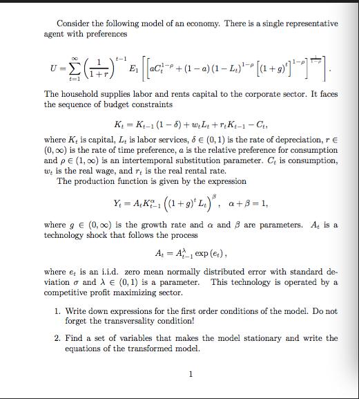
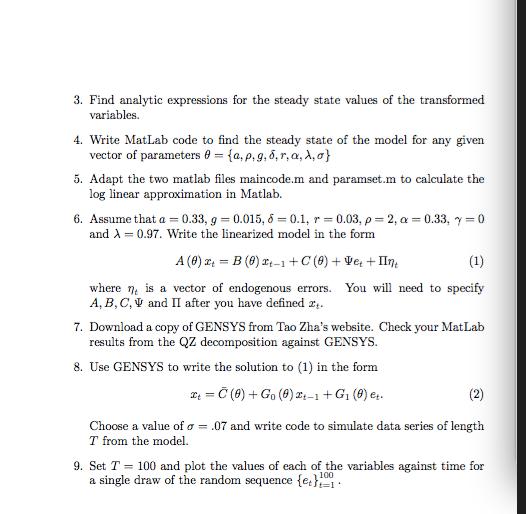
Consider the following model of an economy. There is a single representative agent with preferences 1-p U= - (+)^ E [[aC`* + (1 - 0) (1 L,)~* [(1 + 9)']`~*]**]. t=1 The household supplies labor and rents capital to the corporate sector. It faces the sequence of budget constraints K K-1 (1-6) +wL+rK-1-C where K, is capital, L, is labor services, & (0, 1) is the rate of depreciation, re (0,00) is the rate of time preference, a is the relative preference for consumption and p (1,00) is an intertemporal substitution parameter. Ce is consumption, w is the real wage, and r, is the real rental rate. The production function is given by the expression Y = AK_ ((1+9) L) a+3=1 where g (0,00) is the growth rate and a and 3 are parameters. A, is a technology shock that follows the process A = A exp (et), where e, is an i.i.d. zero mean normally distributed error with standard de- viation and A (0, 1) is a parameter. This technology is operated by a competitive profit maximizing sector. 1. Write down expressions for the first order conditions of the model. Do not forget the transversality condition! 2. Find a set of variables that makes the model stationary and write the equations of the transformed model. 1 3. Find analytic expressions for the steady state values of the transformed variables. 4. Write MatLab code to find the steady state of the model for any given vector of parameters = {a,p.g.6,r,a,,a} 5. Adapt the two matlab files maincode.m and paramset.m to calculate the log linear approximation in Matlab. 6. Assume that a = 0.33, g = 0.015, 6-0.1, r=0.03, p=2, a = 0.33, y=0 and A = 0.97. Write the linearized model in the form A (0)=B (0) t-1+C (0) + Vet + Int (1) where is a vector of endogenous errors. You will need to specify A, B, C, V and II after you have defined 2. 7. Download a copy of GENSYS from Tao Zha's website. Check your MatLab results from the QZ decomposition against GENSYS. 8. Use GENSYS to write the solution to (1) in the form x=C (0) + Go (0) 2-1+G (0) et. (2) Choose a value of a = .07 and write code to simulate data series of length T from the model. 9. Set T 100 and plot the values of each of the variables against time for a single draw of the random sequence {et}=1 1100 Consider the following model of an economy. There is a single representative agent with preferences 1-p U= - (+)^ E [[aC`* + (1 - 0) (1 L,)~* [(1 + 9)']`~*]**]. t=1 The household supplies labor and rents capital to the corporate sector. It faces the sequence of budget constraints K K-1 (1-6) +wL+rK-1-C where K, is capital, L, is labor services, & (0, 1) is the rate of depreciation, re (0,00) is the rate of time preference, a is the relative preference for consumption and p (1,00) is an intertemporal substitution parameter. Ce is consumption, w is the real wage, and r, is the real rental rate. The production function is given by the expression Y = AK_ ((1+9) L) a+3=1 where g (0,00) is the growth rate and a and 3 are parameters. A, is a technology shock that follows the process A = A exp (et), where e, is an i.i.d. zero mean normally distributed error with standard de- viation and A (0, 1) is a parameter. This technology is operated by a competitive profit maximizing sector. 1. Write down expressions for the first order conditions of the model. Do not forget the transversality condition! 2. Find a set of variables that makes the model stationary and write the equations of the transformed model. 1 3. Find analytic expressions for the steady state values of the transformed variables. 4. Write MatLab code to find the steady state of the model for any given vector of parameters = {a,p.g.6,r,a,,a} 5. Adapt the two matlab files maincode.m and paramset.m to calculate the log linear approximation in Matlab. 6. Assume that a = 0.33, g = 0.015, 6-0.1, r=0.03, p=2, a = 0.33, y=0 and A = 0.97. Write the linearized model in the form A (0)=B (0) t-1+C (0) + Vet + Int (1) where is a vector of endogenous errors. You will need to specify A, B, C, V and II after you have defined 2. 7. Download a copy of GENSYS from Tao Zha's website. Check your MatLab results from the QZ decomposition against GENSYS. 8. Use GENSYS to write the solution to (1) in the form x=C (0) + Go (0) 2-1+G (0) et. (2) Choose a value of a = .07 and write code to simulate data series of length T from the model. 9. Set T 100 and plot the values of each of the variables against time for a single draw of the random sequence {et}=1 1100