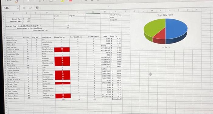
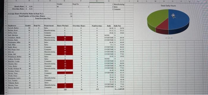
E 5) CHART - Create a 3-D pie chart showing the breakdown of total Hours Worked into total Overtime Hours and the NenQvectime hours located at the bottom of the database listing, row 37 columns E, F, G. The pie chart should show the values, the legend should indicate Overtime Hours and NonQvertime, and the chart title should be Total Daily Hours. Place this chart so that it will fill cells K1:R16. (Hint: When selecting the data for this chart remember that pie charts show parts of a whole so there's no reason to include a total if you are displaying the parts making up that total.) [In spreadsheets, does it make sense to put totals at the bottom of the database?] 6) DATA TABLE - Create a Data Table that shows the average Daily Pay by gender for each department number. Start the criteria in cell E40 and the data table in cell E44. 7) SUBTOTALS - Create a Subtotal showing the total hours worked by department and the total overtime hours worked by gender within each department. Change to Outline View 3 . IWhich department works the most hours and do you see something odd about the overtime hours?1. Copy the subtotal information to Sheet 2 using Copy/Paste Special Values (previously undisplaved/hidden data will appear when copied to Sheet 2). Remove the Subtotaling on Sheet I using the Remove All button before continuing. 8) GOAL SEEK - In cell E7, place a formula that will multiply the Overtime Rate (B3) by the Total Number of Overtime Hours. Perform a Yoal Seek to determine the overtime rate necessary to achieve $400 in total overtime pay. Leave the goal seek in place so that it can be graded. 9) EXTRACT (Advanced Filter) - Sort the database by the employees' names in ascending order. Extract just the name and the department number (Dept. No.) of those who worked more than 8 hours. Start the criteria in cell A40 and the extract output in cell A44. 10) DATA TABLE - on SHEET 3 create a One-Variable Data Table that will take the ODD numbers from 1 to 55 and will show each of the following independent calculations: multiply by 5) CHART - Create a 3-D pie chart showing the breakdown of total Hours Worked into total Overtime Hours and the NonQvectime hours located at the bottom of the database listing, row 37 columns E, F, G. The pie chart should show the values, the legend should indicate Overtime Hours and NonQvertime, and the chart title should be Total Daily Hours. Place this chart so that it will fill cells K1:R16. (Hint: When selecting the data for this chart remember that pie charts show parts of a whole so there's no reason to include a total if you are displaying the parts making up that total.) [In spreadsheets, does it make sense to put totals at the bottom of the database?] 6) DATA TABLE - Create a Data Table that shows the average Daily Pay by gender for each department number. Start the criteria in cell E40 and the data table in cell E44. 7) SUBTOTALS - Create a Subtotal showing the total hours worked by department and the total overtime hours worked by gender within each department. Change to Outline View 3 . [Which department works the most hours and do you see something odd about the overtime hours?] Copy the subtotal information to Sheet 2 using Copy/Paste Special Values (previously undisploxed/hidden data will appear when copied to Sheet 2 ). Remove the Subtotaling on Sheet I using the Remove All button before continuing. 8) GOAL SEEK - In cell E7, place a formula that will multiply fhe Overtime Rate (B3) by the Total Number of Overtime Hours. Perform a Goal Seek to determine the overtime rate necessary to achieve $400 in total overtime pay. Leave the goal seek in place so that it can be graded. 9) EXTRACT (Advanced Filter) - Sort the database by the employees' names in ascending order. Extract just the name and the department number (Dept. No.) of those who worked more than 8 hours. Start the criteria in cell A40 and the extract output in cell A44. 10) DATA TABLE - on SHEET 3 create a One-Variable Data Table that will take the ODD numbers from 1 to 55 and will show each of the following independent calculations: multiply by $6.64; divide by 3.245 ; add $8.23 to each number; subtract 4 from each number. 11) Put your name in the Header and submit your file (instructor's flash drive or Blackboard). 12) If required by your instructor, print the Sheet I worksheet (including chart) landscape orientation, showing the worksheet frame (row \& column headings), fit-to-one page. If required, print the contents of Sheet 2 and Sheet 3. E 5) CHART - Create a 3-D pie chart showing the breakdown of total Hours Worked into total Overtime Hours and the NenQvectime hours located at the bottom of the database listing, row 37 columns E, F, G. The pie chart should show the values, the legend should indicate Overtime Hours and NonQvertime, and the chart title should be Total Daily Hours. Place this chart so that it will fill cells K1:R16. (Hint: When selecting the data for this chart remember that pie charts show parts of a whole so there's no reason to include a total if you are displaying the parts making up that total.) [In spreadsheets, does it make sense to put totals at the bottom of the database?] 6) DATA TABLE - Create a Data Table that shows the average Daily Pay by gender for each department number. Start the criteria in cell E40 and the data table in cell E44. 7) SUBTOTALS - Create a Subtotal showing the total hours worked by department and the total overtime hours worked by gender within each department. Change to Outline View 3 . IWhich department works the most hours and do you see something odd about the overtime hours?1. Copy the subtotal information to Sheet 2 using Copy/Paste Special Values (previously undisplaved/hidden data will appear when copied to Sheet 2). Remove the Subtotaling on Sheet I using the Remove All button before continuing. 8) GOAL SEEK - In cell E7, place a formula that will multiply the Overtime Rate (B3) by the Total Number of Overtime Hours. Perform a Yoal Seek to determine the overtime rate necessary to achieve $400 in total overtime pay. Leave the goal seek in place so that it can be graded. 9) EXTRACT (Advanced Filter) - Sort the database by the employees' names in ascending order. Extract just the name and the department number (Dept. No.) of those who worked more than 8 hours. Start the criteria in cell A40 and the extract output in cell A44. 10) DATA TABLE - on SHEET 3 create a One-Variable Data Table that will take the ODD numbers from 1 to 55 and will show each of the following independent calculations: multiply by 5) CHART - Create a 3-D pie chart showing the breakdown of total Hours Worked into total Overtime Hours and the NonQvectime hours located at the bottom of the database listing, row 37 columns E, F, G. The pie chart should show the values, the legend should indicate Overtime Hours and NonQvertime, and the chart title should be Total Daily Hours. Place this chart so that it will fill cells K1:R16. (Hint: When selecting the data for this chart remember that pie charts show parts of a whole so there's no reason to include a total if you are displaying the parts making up that total.) [In spreadsheets, does it make sense to put totals at the bottom of the database?] 6) DATA TABLE - Create a Data Table that shows the average Daily Pay by gender for each department number. Start the criteria in cell E40 and the data table in cell E44. 7) SUBTOTALS - Create a Subtotal showing the total hours worked by department and the total overtime hours worked by gender within each department. Change to Outline View 3 . [Which department works the most hours and do you see something odd about the overtime hours?] Copy the subtotal information to Sheet 2 using Copy/Paste Special Values (previously undisploxed/hidden data will appear when copied to Sheet 2 ). Remove the Subtotaling on Sheet I using the Remove All button before continuing. 8) GOAL SEEK - In cell E7, place a formula that will multiply fhe Overtime Rate (B3) by the Total Number of Overtime Hours. Perform a Goal Seek to determine the overtime rate necessary to achieve $400 in total overtime pay. Leave the goal seek in place so that it can be graded. 9) EXTRACT (Advanced Filter) - Sort the database by the employees' names in ascending order. Extract just the name and the department number (Dept. No.) of those who worked more than 8 hours. Start the criteria in cell A40 and the extract output in cell A44. 10) DATA TABLE - on SHEET 3 create a One-Variable Data Table that will take the ODD numbers from 1 to 55 and will show each of the following independent calculations: multiply by $6.64; divide by 3.245 ; add $8.23 to each number; subtract 4 from each number. 11) Put your name in the Header and submit your file (instructor's flash drive or Blackboard). 12) If required by your instructor, print the Sheet I worksheet (including chart) landscape orientation, showing the worksheet frame (row \& column headings), fit-to-one page. If required, print the contents of Sheet 2 and Sheet 3


