ex3x.dat:

 2.1040000e+03 3.0000000e+00 1.6000000e+03 3.0000000e+00 2.4000000e+03 3.0000000e+00 1.4160000e+03 2.0000000e+00 3.0000000e+03 4.0000000e+00 1.9850000e+03 4.0000000e+00 1.5340000e+03 3.0000000e+00 1.4270000e+03 3.0000000e+00 1.3800000e+03 3.0000000e+00 1.4940000e+03 3.0000000e+00 1.9400000e+03 4.0000000e+00 2.0000000e+03 3.0000000e+00 1.8900000e+03 3.0000000e+00 4.4780000e+03 5.0000000e+00 1.2680000e+03 3.0000000e+00 2.3000000e+03 4.0000000e+00 1.3200000e+03 2.0000000e+00 1.2360000e+03 3.0000000e+00 2.6090000e+03 4.0000000e+00 3.0310000e+03 4.0000000e+00 1.7670000e+03 3.0000000e+00 1.8880000e+03 2.0000000e+00 1.6040000e+03 3.0000000e+00 1.9620000e+03 4.0000000e+00 3.8900000e+03 3.0000000e+00 1.1000000e+03 3.0000000e+00 1.4580000e+03 3.0000000e+00 2.5260000e+03 3.0000000e+00 2.2000000e+03 3.0000000e+00 2.6370000e+03 3.0000000e+00 1.8390000e+03 2.0000000e+00 1.0000000e+03 1.0000000e+00 2.0400000e+03 4.0000000e+00 3.1370000e+03 3.0000000e+00 1.8110000e+03 4.0000000e+00 1.4370000e+03 3.0000000e+00 1.2390000e+03 3.0000000e+00 2.1320000e+03 4.0000000e+00 4.2150000e+03 4.0000000e+00 2.1620000e+03 4.0000000e+00 1.6640000e+03 2.0000000e+00 2.2380000e+03 3.0000000e+00 2.5670000e+03 4.0000000e+00 1.2000000e+03 3.0000000e+00 8.5200000e+02 2.0000000e+00 1.8520000e+03 4.0000000e+00 1.2030000e+03 3.0000000e+00

ex3y.dat:

 3.9990000e+05 3.2990000e+05 3.6900000e+05 2.3200000e+05 5.3990000e+05 2.9990000e+05 3.1490000e+05 1.9899900e+05 2.1200000e+05 2.4250000e+05 2.3999900e+05 3.4700000e+05 3.2999900e+05 6.9990000e+05 2.5990000e+05 4.4990000e+05 2.9990000e+05 1.9990000e+05 4.9999800e+05 5.9900000e+05 2.5290000e+05 2.5500000e+05 2.4290000e+05 2.5990000e+05 5.7390000e+05 2.4990000e+05 4.6450000e+05 4.6900000e+05 4.7500000e+05 2.9990000e+05 3.4990000e+05 1.6990000e+05 3.1490000e+05 5.7990000e+05 2.8590000e+05 2.4990000e+05 2.2990000e+05 3.4500000e+05 5.4900000e+05 2.8700000e+05 3.6850000e+05 3.2990000e+05 3.1400000e+05 2.9900000e+05 1.7990000e+05 2.9990000e+05 2.3950000e+05

gradient3 student_GD.m :

%in this exercise, you will investigate linear regression using gradient descent % and the normal equations %This is a training set of housing prices in Portland, Oregon, where %y are the prices and the inputs $x are the living area and the number of bedrooms. %we will use only living area in this assigment % initialize samples of x and y training dataset % x2 = load('ex3x.dat'); y = load('ex3y.dat'); %house cost x=x2(:,1); %only living area m = length(y); % store the number of training examples x = [ones(m, 1), x]; % Add a column of ones to x %the area values from your training data are actually in the second column of x #Gradient descent xorg=x(:,2); #normilze the data sigma = std(x); mu = mean(x); x(:,2) = (x(:,2) - mu(2))./ sigma(2); mse = zeros(100, 100); % initialize mse to 100x100 matrix of 0's w0 = linspace(100000,500000,100); w1 = linspace(1000,300000,100); for i = 1:length(w0) for j = 1:length(w1) t = [w0(i); w1(j)]; mse(i,j) =1/m* (y-x*t)'*(y-x*t); end end % Plot the surface plot % Because of the way meshgrids work in the surf command, we need to % transpose mse before calling surf, or else the axes will be flipped mse = mse'; figure; surf(w0, w1, mse); xlabel('\w0'); ylabel('\w1'); w = zeros(2, 1); iterations = 100 alpha = 0.07 cost=zeros(iterations,1); for iter = 1:iterations %insert your code here % cost(iter)=... % this is the code to calculate weights % w=w - your code * alpha; %end of your code wdraw0(iter)=w(1); wdraw1(iter)=w(2); end disp("w0g w1g"),disp(w); % now plot Cost % technically, the first cost at the zero-eth iteration % but Matlab/Octave doesn't have a zero index figure; plot(0:iterations-1, cost(1:iterations), '-') xlabel('Number of iterations') ylabel('Cost - mean square error ') #normilize 1650sf %caling 1650sf your code here: %newxs= your code newxs= disp("house prediction for 1650s, gradient descent:"),disp([1,newxs]*w); #plot data and regression line figure % open a new figure window # plot your training set (and label the axes): plot(xorg,y,'o'); ylabel('house cost') xlabel('house sf') hold yp=x*w; plot(xorg,yp,'-'); 

gradient3student_neq.m :

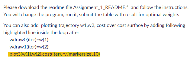
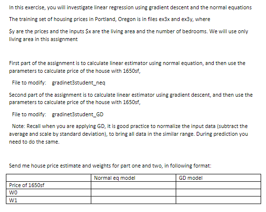
%in this exercise, you will investigate linear regression using gradient descent % and the normal equations %This is a training set of housing prices in Portland, Oregon, where %y are the prices and the inputs $x are the living area and the number of bedrooms. %we will use only living area in this assigment % initialize samples of x and y training dataset % x2 = load('ex3x.dat'); y = load('ex3y.dat'); %house cost x=x2(:,1); %only living area m = length(y); % store the number of training examples x = [ones(m, 1), x]; % Add a column of ones to x %the area values from your training data are actually in the second column of x %calculate parametar w using normal equation %your code here % %w= %code end disp("w0 w1"),disp(wn); #predict the house price with 1650sf disp("house prediction for 1650s, normal eq:"),disp([1,1650]*wn); yp=x*wn; #plot data and regression line figure % open a new figure window # plot your training set (and label the axes): plot(x(:,2),y,'o'); ylabel('house cost') xlabel('house sf') hold plot(x(:,2),yp,'-'); Please help using octave(mathlab) for programming step by step for understanding and the files (can be used). Question is for linear regression using gradient descent. I need understanding on how to modify the script(code). Thank you 

Please download the readme file Assignment_1_README.* and follow the instructions. You will change the program, run it, submit the table with result for optimal weights You can also add plotting trajectory w1,w2, cost over cost surface by adding following highlighted line inside the loop after wdrawO( iter )=w(1); wdraw 1( iter )=w(2) plot3(w(1),w(2),cost(iter),'rv",'markersize',10) The training set of housing prices in Portland, Oregon is in files ex3x and ex3y, where Sy are the prices and the inputs $x are the living area and the number of bedrooms. We will use only living area in this assignment First part of the assignment is to calculate linear estimator using normal equation, and then use the parameters to calculate price of the house with 1650 sf, File to modify: gradinet3student_neq Second part of the assignment is to calculate linear estimator using gradient descent, and then use the parameters to calculate price of the house with 1650 sf, File to modify: gradinet3student_GD Note: Recall when you are applying GD, it is good practice to normalize the input data (subtract the average and scale by standard deviation), to bring all data in the similar range. During prediction you need to do the same. Send me house price estimate and weights for part one and two, in following format: Please download the readme file Assignment_1_README.* and follow the instructions. You will change the program, run it, submit the table with result for optimal weights You can also add plotting trajectory w1,w2, cost over cost surface by adding following highlighted line inside the loop after wdrawO( iter )=w(1); wdraw 1( iter )=w(2) plot3(w(1),w(2),cost(iter),'rv",'markersize',10) The training set of housing prices in Portland, Oregon is in files ex3x and ex3y, where Sy are the prices and the inputs $x are the living area and the number of bedrooms. We will use only living area in this assignment First part of the assignment is to calculate linear estimator using normal equation, and then use the parameters to calculate price of the house with 1650 sf, File to modify: gradinet3student_neq Second part of the assignment is to calculate linear estimator using gradient descent, and then use the parameters to calculate price of the house with 1650 sf, File to modify: gradinet3student_GD Note: Recall when you are applying GD, it is good practice to normalize the input data (subtract the average and scale by standard deviation), to bring all data in the similar range. During prediction you need to do the same. Send me house price estimate and weights for part one and two, in following format