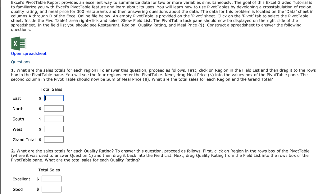
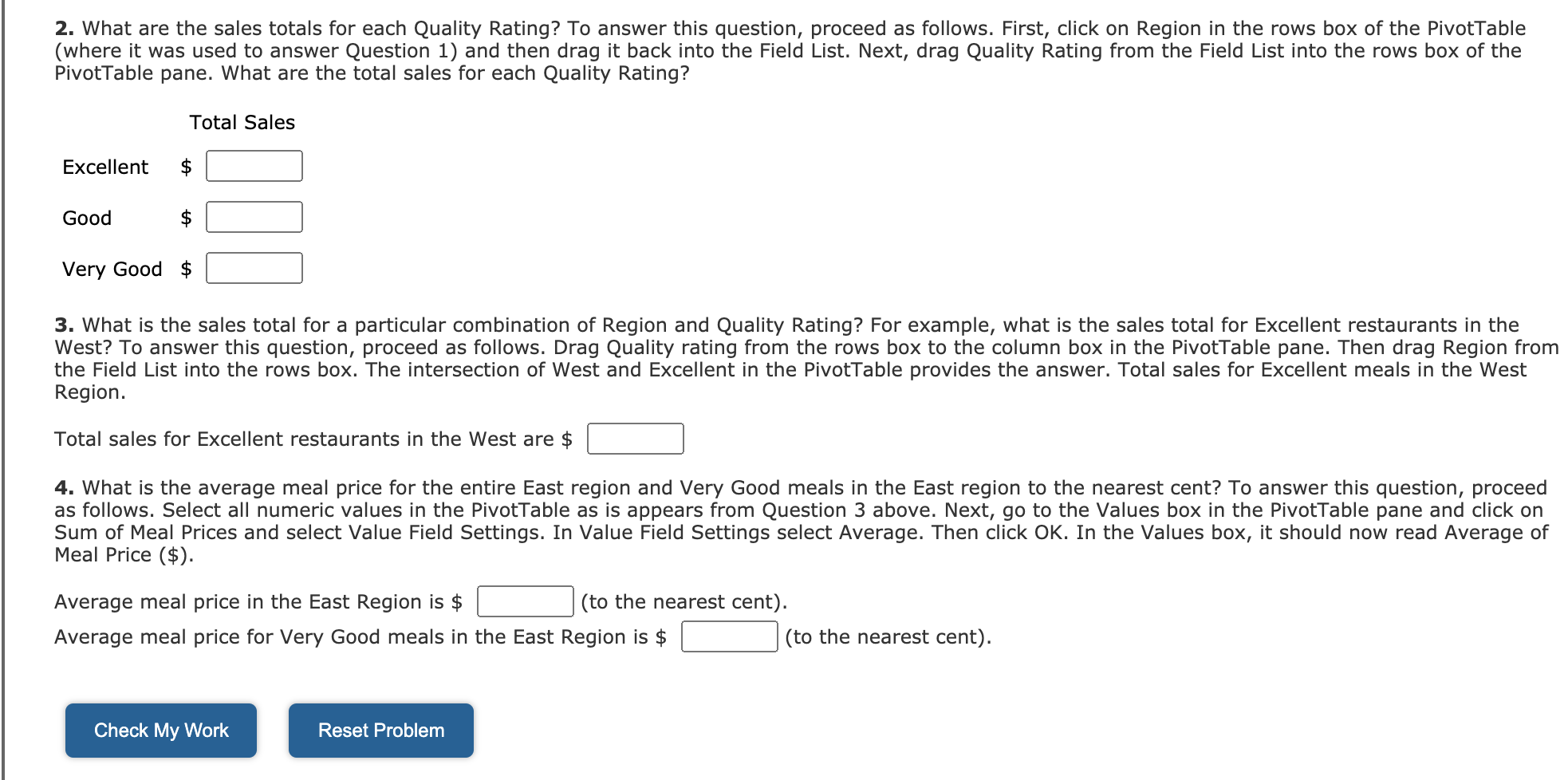
Excel's PivotTable Report provides an excellent way to summarize data for two or more variables simultaneously. The goal of this Excel Graded Tutorial is to familiarize you with Excel's Pivottable feature and learn about its uses. You will learn how to use PivotTables by developing a crosstabulation of region, quality rating, and meal price for 300 restaurants and then answering questions about the data. The data for this problem is located on the 'Data' sheet in columns A through D of the Excel Online file below. An empty PivotTable is provided on the 'Pivot' sheet. Click on the 'Pivot' tab to select the PivotTable sheet. Inside the PivotTable1 area right-click and select Show Field List. The PivotTable task pane should now be displayed on the right side of the spreadsheet. In the field list you should see Restaurant, Region, Quality Rating, and Meal Price ($). Construct a spreadsheet to answer the following questions. Open spreadsheet Questions 1. What are the sales totals for each region? To answer this question, proceed as follows. First, click on Region in the Field List and then drag it to the rows box in the Pivot Table pane. You will see the four regions enter the Pivottable. Next, drag Meal Price ($) into the values box of the PivotTable pane. The second column in the Pivot Table should now be Sum of Meal Price ($). What are the total sales for each Region and the Grand Total? Total Sales East $ North $ South $ West $ Grand Total $ 2. What are the sales totals for each Quality Rating? To answer this question, proceed as follows. First, click on Region in the rows box of the PivotTable (where it was used to answer Question 1) and then drag it back into the Field List. Next, drag Quality Rating from the Field List into the rows box of the PivotTable pane. What are the total sales for each Quality Rating? Total Sales Excellent $ Good $ 2. What are the sales totals for each Quality Rating? To answer this question, proceed as follows. First, click on Region in the rows box of the PivotTable (where it was used to answer Question 1) and then drag it back into the Field List. Next, drag Quality Rating from the Field List into the rows box of the PivotTable pane. What are the total sales for each Quality Rating? Total Sales Excellent Good Very Good $ 3. What is the sales total for a particular combination of Region and Quality Rating? For example, what is the sales total for Excellent restaurants in the West? To answer this question, proceed as follows. Drag Quality rating from the rows box to the column box in the PivotTable pane. Then drag Region from the Field List into the rows box. The intersection of West and Excellent in the Pivottable provides the answer. Total sales for Excellent meals in the West Region. Total sales for Excellent restaurants in the West are $ 4. What is the average meal price for the entire East region and Very Good meals in the East region to the nearest cent? To answer this question, proceed as follows. Select all numeric values in the PivotTable as is appears from Question 3 above. Next, go to the Values box in the PivotTable pane and click on Sum of Meal Prices and select Value Field Settings. In Value Field Settings select Average. Then click OK. In the Values box, it should now read Average of Meal Price ($). Average meal price in the East Region is $ (to the nearest cent). Average meal price for Very Good meals in the East Region is $ (to the nearest cent). Check My Work Reset Problem Excel's PivotTable Report provides an excellent way to summarize data for two or more variables simultaneously. The goal of this Excel Graded Tutorial is to familiarize you with Excel's Pivottable feature and learn about its uses. You will learn how to use PivotTables by developing a crosstabulation of region, quality rating, and meal price for 300 restaurants and then answering questions about the data. The data for this problem is located on the 'Data' sheet in columns A through D of the Excel Online file below. An empty PivotTable is provided on the 'Pivot' sheet. Click on the 'Pivot' tab to select the PivotTable sheet. Inside the PivotTable1 area right-click and select Show Field List. The PivotTable task pane should now be displayed on the right side of the spreadsheet. In the field list you should see Restaurant, Region, Quality Rating, and Meal Price ($). Construct a spreadsheet to answer the following questions. Open spreadsheet Questions 1. What are the sales totals for each region? To answer this question, proceed as follows. First, click on Region in the Field List and then drag it to the rows box in the Pivot Table pane. You will see the four regions enter the Pivottable. Next, drag Meal Price ($) into the values box of the PivotTable pane. The second column in the Pivot Table should now be Sum of Meal Price ($). What are the total sales for each Region and the Grand Total? Total Sales East $ North $ South $ West $ Grand Total $ 2. What are the sales totals for each Quality Rating? To answer this question, proceed as follows. First, click on Region in the rows box of the PivotTable (where it was used to answer Question 1) and then drag it back into the Field List. Next, drag Quality Rating from the Field List into the rows box of the PivotTable pane. What are the total sales for each Quality Rating? Total Sales Excellent $ Good $ 2. What are the sales totals for each Quality Rating? To answer this question, proceed as follows. First, click on Region in the rows box of the PivotTable (where it was used to answer Question 1) and then drag it back into the Field List. Next, drag Quality Rating from the Field List into the rows box of the PivotTable pane. What are the total sales for each Quality Rating? Total Sales Excellent Good Very Good $ 3. What is the sales total for a particular combination of Region and Quality Rating? For example, what is the sales total for Excellent restaurants in the West? To answer this question, proceed as follows. Drag Quality rating from the rows box to the column box in the PivotTable pane. Then drag Region from the Field List into the rows box. The intersection of West and Excellent in the Pivottable provides the answer. Total sales for Excellent meals in the West Region. Total sales for Excellent restaurants in the West are $ 4. What is the average meal price for the entire East region and Very Good meals in the East region to the nearest cent? To answer this question, proceed as follows. Select all numeric values in the PivotTable as is appears from Question 3 above. Next, go to the Values box in the PivotTable pane and click on Sum of Meal Prices and select Value Field Settings. In Value Field Settings select Average. Then click OK. In the Values box, it should now read Average of Meal Price ($). Average meal price in the East Region is $ (to the nearest cent). Average meal price for Very Good meals in the East Region is $ (to the nearest cent). Check My Work Reset