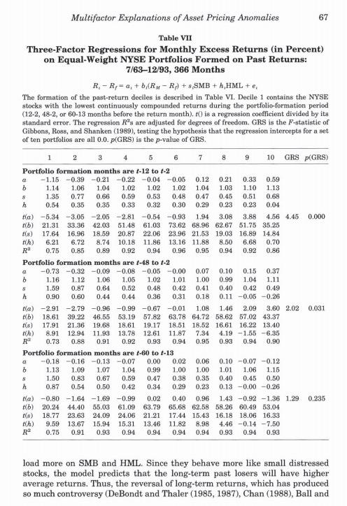
Fama and French (1996) Table VII reports regression results for the Fama and French (1993) 3-factor model [FF3] against trend-based portfolio strategies. i) Briefly describe a contrarian strategy and a momentum strategy. ii) How does the FF3 model perform against both trading strategies in i)? iii) Can FF3 explain the return of a contrarian portfolio? Why or why not? iii) Can FF3 explain the return of a momentum portfolio? Why or why not? 67 Multifactor Explanations of Asset Pricing Anomalies Table VII Three-Factor Regressions for Monthly Excess Returns (in Percent) on Equal-Weight NYSE Portfolios Formed on Past Returns: 7/63-12/93, 366 Months R. - R = , + BARN - Rp) + s SMB + h HML +, The formation of the past-return deciles is described in Table VI. Decile 1 contains the NYSE stocks with the lowest continuously compounded returns during the portfolio-formation period (12-2, 48-2, or 60-13 months before the return month). O is a regression coefficient divided by its standard error. The regression R's are adjusted for degrees of freedom. GRS is the P-statistic of Gibbons, Ross, and Shanken (1989), testing the hypothesis that the regression intercepts for a set of ten portfolios are all 0.0.p(GRS) is the p-value of GRS. 1 2 3 4 8 9 10 GRS p(GRS) Portfolio formation months are t-12 to 1-2 a -1.15 -0.39 -0.21 -0.22 -0.04 -0.05 0.12 0.21 0.33 0.59 1.14 1.06 1.04 1.02 1.02 1.02 1.04 1.03 1.10 1.13 8 1.35 0.77 0.66 0.59 0.53 0.48 0.47 0.45 0.51 0.68 h 0.54 0.35 0.35 0.33 0.32 0.30 0.29 0.23 0.23 0.04 tla) -5.34 -3.05 -2.05 -2.81 -0.54 -0.93 1.94 3.08 3.88 4.56 4.45 0.000 Mb) 21.31 33.36 42.03 51.48 61.03 73.62 68.96 62.67 51.75 35.25 tis) 17.64 16.96 18.59 20.87 22.06 23.96 21.53 19.03 16.89 14.84 th) 6.21 6.72 8.74 10.18 11.86 13.16 11.88 8.50 6.68 0.70 0.75 0.85 0.89 0.92 0.94 0.96 0.95 0.94 0.92 0.86 Portfolio formation months are 1-48 to 1-2 a -0.73 -0.32 -0.09 -0.08 -0.05 -0.00 0.07 0.10 0.15 0.37 b 1.16 1.12 1.06 1.05 1.02 1.01 1.00 0.99 1.04 1.11 S 1.59 0.87 0.64 0.52 0.48 0.42 0.41 0.40 0.42 0.49 h 0.90 0.60 0.44 0.44 0.36 0.31 0.18 0.11 -0.05 -0.26 tla) -2.91 -2.79 -0.96 -0.99 -0.67 -0.01 1.08 1.46 2.09 3.60 2.02 0.031 b) 18.61 39.22 46.56 53.19 57.82 63.78 64.72 58.62 57.02 43.37 tis) 17.91 21.36 19.68 18.61 19.17 18.51 18.52 16.61 16.22 13.40 (h) 8.91 12.94 11.93 13.78 12.61 11.87 7.34 4.19 -1.55 -6.35 R 0.73 0.88 0.91 0.92 0.93 0.94 0.95 0.93 0.94 0.90 Portfolio formation months are +-60 to 1-13 a -0.18-0.16 -0.13-0.07 0.00 0.02 0.06 0.10 -0.07 -0.12 b 1.13 1.09 1.07 1.04 0.99 1.00 1.00 1.01 1.06 1.15 s 1.50 0.83 0.67 0.59 0.47 0.38 0.35 0.40 0.45 0.50 h 0.87 0.54 0.50 0.42 0.34 0.29 0.23 0.13 -0.00 -0.26 ka) -0.80 -1.64 -1.69 -0.99 0.02 0.40 0.96 1.43 -0.92 -1.36 1.29 0.235 b) 20.24 44.40 55.03 61.09 63.79 65.68 62.58 58.26 60.49 53.04 (8) 18.77 23.63 24.09 24.06 21.21 17.44 15.43 16.18 18.06 16.33 th) 9.59 13.67 15.94 15.31 13.46 11.82 8.98 4.46 -0.14 -7.50 R 0.75 0.91 0.93 0.94 0.94 0.94 0.94 0.93 0.94 0.93 load more on SMB and HML. Since they behave more like small distressed stocks, the model predicts that the long-term past losers will have higher average returns. Thus, the reversal of long-term returns, which has produced so much controversy (DeBondt and Thaler (1985, 1987), Chan (1988), Ball and Fama and French (1996) Table VII reports regression results for the Fama and French (1993) 3-factor model [FF3] against trend-based portfolio strategies. i) Briefly describe a contrarian strategy and a momentum strategy. ii) How does the FF3 model perform against both trading strategies in i)? iii) Can FF3 explain the return of a contrarian portfolio? Why or why not? iii) Can FF3 explain the return of a momentum portfolio? Why or why not? 67 Multifactor Explanations of Asset Pricing Anomalies Table VII Three-Factor Regressions for Monthly Excess Returns (in Percent) on Equal-Weight NYSE Portfolios Formed on Past Returns: 7/63-12/93, 366 Months R. - R = , + BARN - Rp) + s SMB + h HML +, The formation of the past-return deciles is described in Table VI. Decile 1 contains the NYSE stocks with the lowest continuously compounded returns during the portfolio-formation period (12-2, 48-2, or 60-13 months before the return month). O is a regression coefficient divided by its standard error. The regression R's are adjusted for degrees of freedom. GRS is the P-statistic of Gibbons, Ross, and Shanken (1989), testing the hypothesis that the regression intercepts for a set of ten portfolios are all 0.0.p(GRS) is the p-value of GRS. 1 2 3 4 8 9 10 GRS p(GRS) Portfolio formation months are t-12 to 1-2 a -1.15 -0.39 -0.21 -0.22 -0.04 -0.05 0.12 0.21 0.33 0.59 1.14 1.06 1.04 1.02 1.02 1.02 1.04 1.03 1.10 1.13 8 1.35 0.77 0.66 0.59 0.53 0.48 0.47 0.45 0.51 0.68 h 0.54 0.35 0.35 0.33 0.32 0.30 0.29 0.23 0.23 0.04 tla) -5.34 -3.05 -2.05 -2.81 -0.54 -0.93 1.94 3.08 3.88 4.56 4.45 0.000 Mb) 21.31 33.36 42.03 51.48 61.03 73.62 68.96 62.67 51.75 35.25 tis) 17.64 16.96 18.59 20.87 22.06 23.96 21.53 19.03 16.89 14.84 th) 6.21 6.72 8.74 10.18 11.86 13.16 11.88 8.50 6.68 0.70 0.75 0.85 0.89 0.92 0.94 0.96 0.95 0.94 0.92 0.86 Portfolio formation months are 1-48 to 1-2 a -0.73 -0.32 -0.09 -0.08 -0.05 -0.00 0.07 0.10 0.15 0.37 b 1.16 1.12 1.06 1.05 1.02 1.01 1.00 0.99 1.04 1.11 S 1.59 0.87 0.64 0.52 0.48 0.42 0.41 0.40 0.42 0.49 h 0.90 0.60 0.44 0.44 0.36 0.31 0.18 0.11 -0.05 -0.26 tla) -2.91 -2.79 -0.96 -0.99 -0.67 -0.01 1.08 1.46 2.09 3.60 2.02 0.031 b) 18.61 39.22 46.56 53.19 57.82 63.78 64.72 58.62 57.02 43.37 tis) 17.91 21.36 19.68 18.61 19.17 18.51 18.52 16.61 16.22 13.40 (h) 8.91 12.94 11.93 13.78 12.61 11.87 7.34 4.19 -1.55 -6.35 R 0.73 0.88 0.91 0.92 0.93 0.94 0.95 0.93 0.94 0.90 Portfolio formation months are +-60 to 1-13 a -0.18-0.16 -0.13-0.07 0.00 0.02 0.06 0.10 -0.07 -0.12 b 1.13 1.09 1.07 1.04 0.99 1.00 1.00 1.01 1.06 1.15 s 1.50 0.83 0.67 0.59 0.47 0.38 0.35 0.40 0.45 0.50 h 0.87 0.54 0.50 0.42 0.34 0.29 0.23 0.13 -0.00 -0.26 ka) -0.80 -1.64 -1.69 -0.99 0.02 0.40 0.96 1.43 -0.92 -1.36 1.29 0.235 b) 20.24 44.40 55.03 61.09 63.79 65.68 62.58 58.26 60.49 53.04 (8) 18.77 23.63 24.09 24.06 21.21 17.44 15.43 16.18 18.06 16.33 th) 9.59 13.67 15.94 15.31 13.46 11.82 8.98 4.46 -0.14 -7.50 R 0.75 0.91 0.93 0.94 0.94 0.94 0.94 0.93 0.94 0.93 load more on SMB and HML. Since they behave more like small distressed stocks, the model predicts that the long-term past losers will have higher average returns. Thus, the reversal of long-term returns, which has produced so much controversy (DeBondt and Thaler (1985, 1987), Chan (1988), Ball and