Answered step by step
Verified Expert Solution
Link Copied!

Question

1 Approved Answer

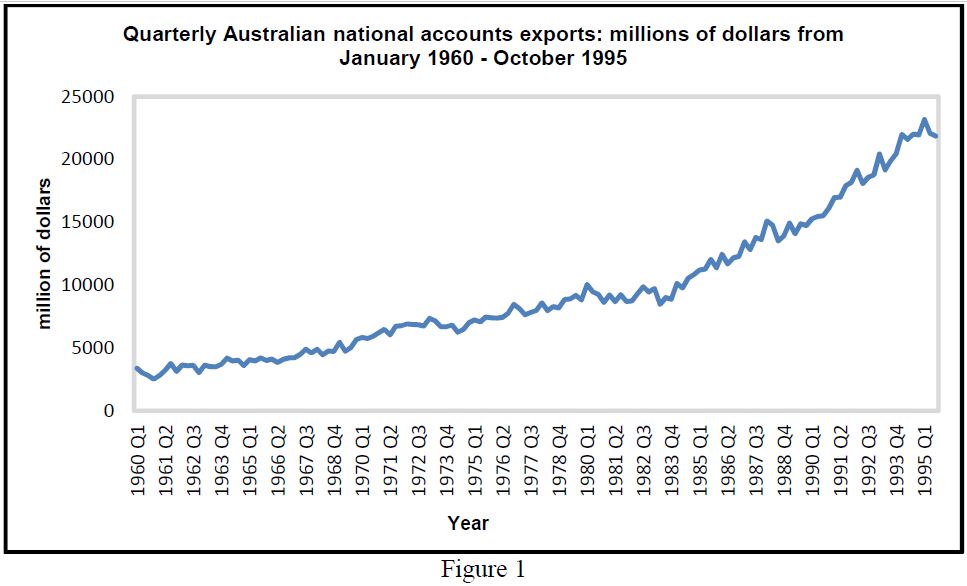
Figure 1 shows the quarterly exports of Australian national accounts from January 1960 - October 1995. Regression Statistics Multiple R 0.945466 R Square 0.893907 Adjusted

Figure 1 shows the quarterly exports of Australian national accounts from January 1960 -

October 1995.
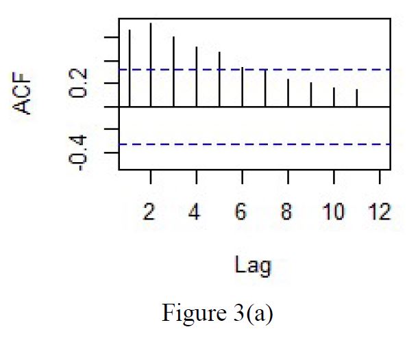
image text in transcribedimage text in transcribedimage text in transcribedimage text in transcribedimage text in transcribedimage text in transcribedimage text in transcribed
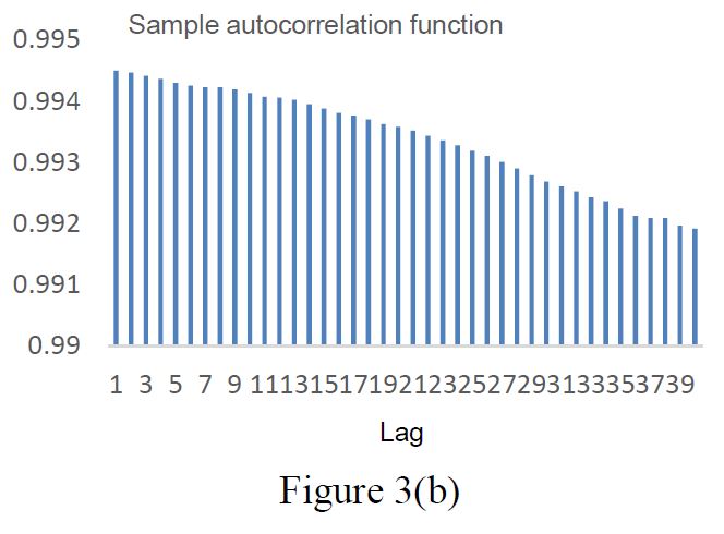
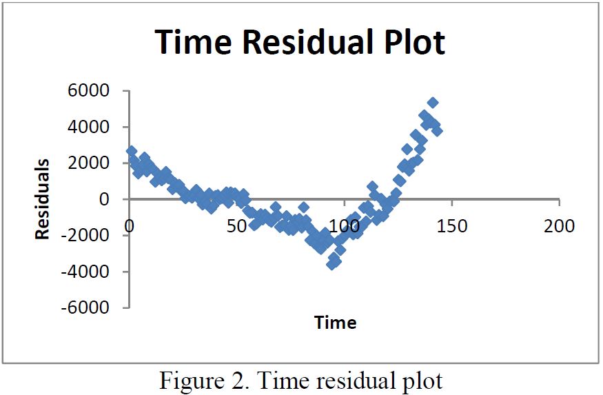
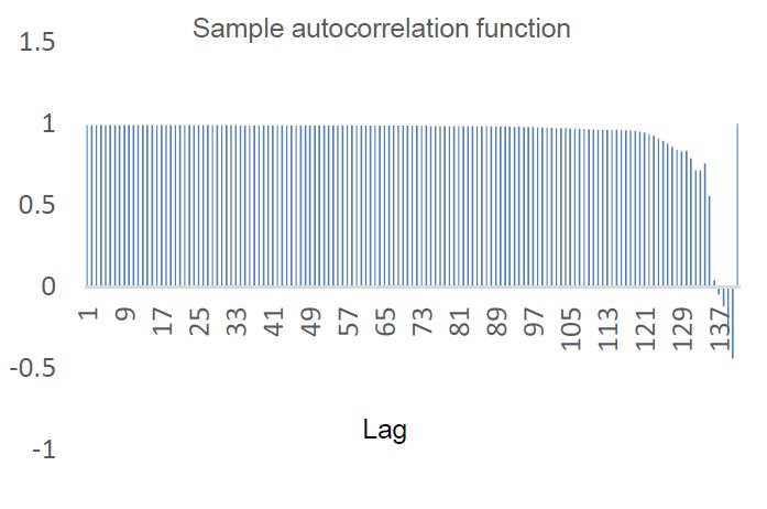
Regression Statistics Multiple R 0.945466 R Square 0.893907 Adjusted R Square 0.893154 Standard Error 1751.420 Observations 143 ANOVA SS MS F Significance F Regression 1 364422746 36442274 1188.022 1.450E-70 Residual 141 432513645 3067472 Total 142 4076741109 Coefficients Standard Error t Stat P-value Lower 95% Upper 95% Lower 95.0% Upper 95.0% Intercept 599.0078 294.4652 2.034222 0.043804 16.87018 1181.145578 16.87018067 1181.145578 Time 122.2925 3.548032 34.46770 1.450E-70 115.2783 129.30674 115.2783122 129.3067448 Table 1. Regression analysis resultsACF -0.4 0.2 2 4 6 8 10 12 Lag Figure 3(a)million of dollars 15000 20000 25000 10000 5000 0 1960 Q1 1961 Q2 1962 Q3 1963 Q4 1965 Q1 1966 Q2 1967 Q3 1968 Q4 1970 Q1 1971 Q2 1972 Q3 1973 Q4 Year 1975 Q1 January 1960 - October 1995 Quarterly Australian national accounts exports: millions of dollars from Figure 1 1976 Q2 1977 Q3 1978 Q4 1980 Q1 1981 Q2 1982 Q3 1983 Q4 1985 Q1 1986 Q2 1987 Q3 1988 Q4 1990 Q1 1991 Q2 1992 Q3 1993 Q4 1995 Q1Regression Statistics Multiple R 0.98555305 R Square 0.97 131482 Adjusted R Square 0.97090503 Standard Error 913.947609 Observations 143 ANOVA f SS MS F Significance F Regression 2 3959799077 1979899538 2370.28 1.086E-108 Residual 140 116942032 835300.2326 Total 142 4076741109 Coefficients Standard Error t Stat P-value Lower 95% Upper 95% Lower 95.0% Upper 95.0% Intercept 3991.176 232.5289 17.16421 2.97E-36 3531.454 4450.899 3531.454 4450.899 Time 1 -18.07308 7.455158 -2.424238 0.0166 -32.81232 -3.333832 -32.81232 -3.333832 Time 2 0.974761 0.050149 19.43692 1.35E-41 0.875612 1.073910 0.875612 1.07391 Table 2. Regression analysis results\fTime Residual Plot 6000 4000 2000 O Residuals -2000 50 100 150 200 -4000 -6000 Time Figure 2. Time residual plot1.5 Sample autocorrelation function 0.5 0 113 105 121 137 129 -0.5 Lag -1

Step by Step Solution

There are 3 Steps involved in it

Step: 1

blur-text-image

Get Instant Access to Expert-Tailored Solutions

See step-by-step solutions with expert insights and AI powered tools for academic success

Step: 2

blur-text-image

Step: 3

blur-text-image

Ace Your Homework with AI

Get the answers you need in no time with our AI-driven, step-by-step assistance

Get Started

Recommended Textbook for

Finite Math And Applied Calculus

Authors: Stefan Waner, Steven Costenoble

2nd Edition

0534366309, 9780534366308

More Books

Students also viewed these Mathematics questions

Question

politeness and modesty, as well as indirectness;

Answered: 1 week ago