Fill the next equation to Solve manual solutions please I will appreciate

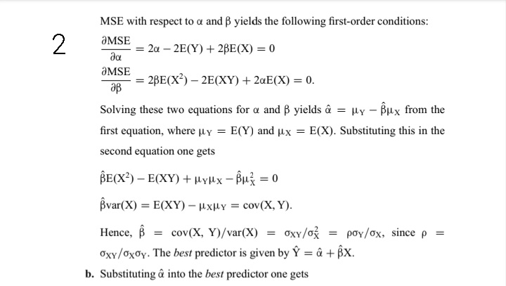
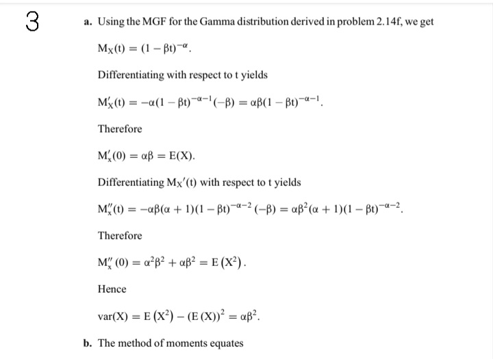
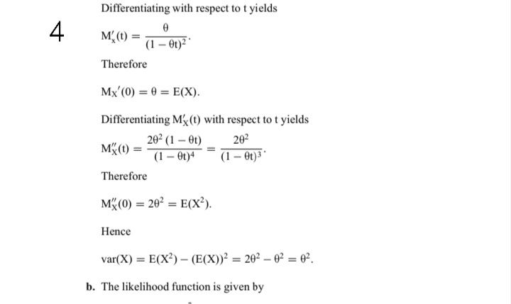
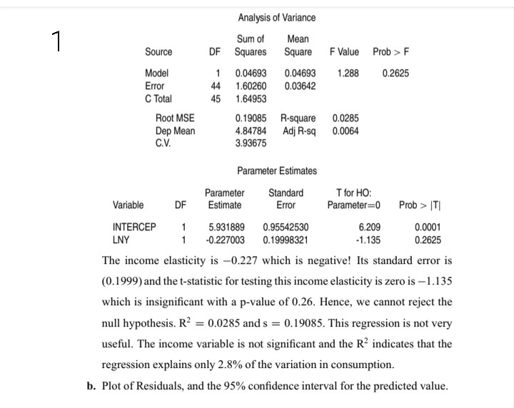
MSE with respect to a and B yields the following first-order conditions: aMSE N = 20 - 2E(Y) + 2BE(X) = 0 da aMSE = 2BE(X-) - 2E(XY) + 2QE(X) = 0. aB Solving these two equations for a and B yields & = My - Bux from the first equation, where uy = E(Y) and ux = E(X). Substituting this in the second equation one gets BE(X2) - E(XY) + HYux -Bu} = 0 Bvar (X) = E(XY) - UXHY = cov(X, Y). Hence, B = cov(X, Y)/var(X) = oxy/ox = poy/ox, since p = Oxy/Oxy. The best predictor is given by Y = & + BX. b. Substituting a into the best predictor one gets3 a. Using the MGF for the Gamma distribution derived in problem 2. 14f, we get Mx (1) = (1 - Bt) . Differentiating with respect to t yields My (t) = -a(1 -Bt) "-'(-B) = aB(1 - Bt) -0-1. Therefore M'(0) = aB = E(X). Differentiating Mx'(t) with respect to t yields M"(t) = -aB(a + 1)(1 -Bt) "-2(-B) = aB2(a+ 1)(1 - Bt) -0-2. Therefore M" (0) = a282 + aB2 = E (X2). Hence var(X) = E (X2) - (E (X))2 = QB2. b. The method of moments equatesDifferentiating with respect to t yields 4 M' (1) = (1 - 0t)2 Therefore Mx'(0) = 0 = E(X). Differentiating My(t) with respect to t yields MY(1) = 202 (1 - 0t) 202 (1 - 0t)4 (1 - 0t)3 Therefore M*(0) = 202 = E(X2 ). Hence var(X) = E(X2) - (E(X) )2 = 202 - 03 = 02. b. The likelihood function is given byAnalysis of Variance Sum of Mean Source DF Squares Square F Value Prob > F Model 1 0.04693 0.04693 1.288 0.2625 Error 44 1.60260 0.03642 C Total 45 1.64953 Root MSE 0.19085 R-square 0.0285 Dep Mean 4.84784 Adj R-sq 0.0064 C.V. 3.93675 Parameter Estimates Parameter Standard T for HO: Variable DF Estimate Error Parameter=0 Prob > [TI INTERCEP 5.931889 0.95542530 6.209 0.0001 LNY -0.227003 0.19998321 -1.135 0.2625 The income elasticity is -0.227 which is negative! Its standard error is (0.1999) and the t-statistic for testing this income elasticity is zero is -1.135 which is insignificant with a p-value of 0.26. Hence, we cannot reject the null hypothesis. R2 = 0.0285 and s = 0.19085. This regression is not very useful. The income variable is not significant and the R indicates that the regression explains only 2.8% of the variation in consumption. b. Plot of Residuals, and the 95% confidence interval for the predicted value