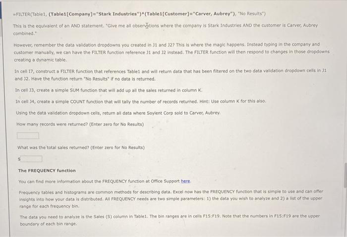
=FILTER(Table 1, (Table1[Company]="Stark Industries ")*(Table 1 Customer]="Carver, Aubrey"), "No Results") This is the equivalent of an AND statement. "Give me all observitions where the company is Stark Industries AND the customer is Carver, Aubrey combined." However, remember the data validation dropdowns you created in J1 and 12? This is where the magic happens. Instead typing in the company and customer manually, we can have the FILTER function reference J1 and 32 instead. The FILTER function will then respond to changes in those dropdowns creating a dynamic table In cell 17, construct a FILTER function that references Tablet and will return data that has been filtered on the two data validation dropdown cells in 31 and 32. Have the function return "No Results" if no data is returned. In cell 3, create a simple SUM function that will add up all the sales returned in column In cell 4, create a simple COUNT function that will tally the number of records returned. Hint: Use column K for this also Using the data validation dropdown cells, return all data where Soylent Corp sold to Carver, Aubrey. How many records were returned? (Enter zero for No Results) What was the total sales returned? (Enter zero for No Results) The FREQUENCY function You can find more information about the FREQUENCY function at Office Support here Frequency tables and histograms are common methods for describing data. Excel now has the FREQUENCY function that is simple to use and can offer Insights into how your data is distributed. All FREQUENCY needs are two simple parameters: 1) the data you wish to analyze and 2) a list of the upper range for each frequency bin The data you need to analyze is the Sales (S) column in Tablel. The bin ranges are in cells F15:F19. Note that the numbers in F15:F19 are the upper boundary of each bin range. =FILTER(Table 1, (Table1[Company]="Stark Industries ")*(Table 1 Customer]="Carver, Aubrey"), "No Results") This is the equivalent of an AND statement. "Give me all observitions where the company is Stark Industries AND the customer is Carver, Aubrey combined." However, remember the data validation dropdowns you created in J1 and 12? This is where the magic happens. Instead typing in the company and customer manually, we can have the FILTER function reference J1 and 32 instead. The FILTER function will then respond to changes in those dropdowns creating a dynamic table In cell 17, construct a FILTER function that references Tablet and will return data that has been filtered on the two data validation dropdown cells in 31 and 32. Have the function return "No Results" if no data is returned. In cell 3, create a simple SUM function that will add up all the sales returned in column In cell 4, create a simple COUNT function that will tally the number of records returned. Hint: Use column K for this also Using the data validation dropdown cells, return all data where Soylent Corp sold to Carver, Aubrey. How many records were returned? (Enter zero for No Results) What was the total sales returned? (Enter zero for No Results) The FREQUENCY function You can find more information about the FREQUENCY function at Office Support here Frequency tables and histograms are common methods for describing data. Excel now has the FREQUENCY function that is simple to use and can offer Insights into how your data is distributed. All FREQUENCY needs are two simple parameters: 1) the data you wish to analyze and 2) a list of the upper range for each frequency bin The data you need to analyze is the Sales (S) column in Tablel. The bin ranges are in cells F15:F19. Note that the numbers in F15:F19 are the upper boundary of each bin range