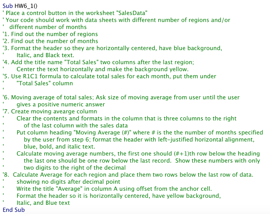
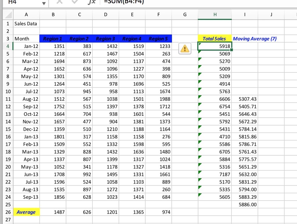
final product should look like this:

this is to be done in VBA!

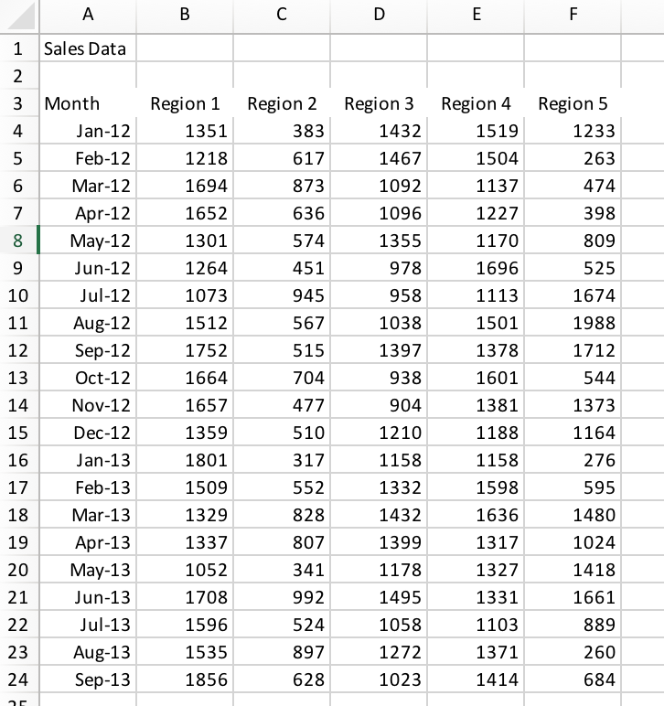
Sub HW6_10 Place a control button in the worksheet "SalesData" Your code should work with data sheets with different number of regions and/or different number of months 1. Find out the number of regions 2. Find out the number of months 3. Format the header so they are horizontally centered, have blue background, Italic, and Black text. Center the text horizontally and make the background yellow Total Sales" column 4. Add the title name "Total Sales" two columns after the last region; 5. Use R1C1 formula to calculate total sales for each month, put them under 6. Moving average of total sales; Ask size of moving average from user until the user 7.Create moving avearge column gives a positive numeric answer Clear the contents and formats in the column that is three columns to the right of the last column with the sales data Put column heading "Moving Average (#)" where # is the the number of months specified by the user from step 6; format the header with left-justified horizontal alignment, blue, bold, and italic text. Calculate moving average numbers, the first one should (#41)th row below the heading the last one should be one row below the last record. Show these numbers with only two digits to the right of the decimal 8. Calculate Average for each region and place them two rows below the last row of data. showing no digits after decimal point Write the title "Average" in column A using offset from the anchor cell. Format the header so it is horizontally centered, have yellow background, Italic, and Blue text End Sub 1 Sales Data 3 Month Region 1 Region 2 Region 3 Region 4 Region 5 1233 263 474 398 809 525 1674 1988 1712 1519 1504 1137 1227 1170 1696 1113 1501 1378 1601 1381 1188 1158 1598 1636 1317 1327 1331 1103 1371 1414 383 1351 1218 1694 1652 1301 1264 1073 1512 1752 1664 1657 1359 1801 1509 1329 1337 1052 1708 1596 1535 1856 1467 1092 1096 1355 Feb-12 873 636 574 451 Mar-12 958 1038 1397 938 904 1210 1158 1332 1432 1399 1178 1495 1058 1272 1023 Jul-12 567 Oct-12 704 1373 1164 276 595 1480 1024 1418 1661 889 260 684 477 Feb-13 Mar-13 552 828 807 992 524 Jul-13 628 1 Sales Data Total Sales Moving Average (7) 3 Month 4 Region 1 Region 2 Region 3 Region 4 Region 5 1519 1504 1137 1227 1170 1696 1113 1501 1378 1601 1381 1188 1158 1598 1636 1317 1327 1331 1103 1371 1414 5918 5069 5270 5009 5209 4914 5763 6606 5307.43 67545405.71 5451 5646.43 5792 5672.29 5431 5784.14 4710 5815.86 5586 5786.71 6705 5761.43 5884 5775.57 5316 5651.29 7187 5632.00 5170 5831.29 5335 5794.00 5605 5883.29 1351 1218 1694 1652 1301 1432 1467 1092 1096 1355 1233 263 809 525 1674 1988 1712 451 1073 1512 1752 567 1038 1397 Oct-12 1657 1359 1801 1509 1329 1337 1052 1708 1596 1535 1856 1373 1210 1158 1332 1432 1399 1178 1495 1058 1272 1023 1164 828 807 1480 1024 1418 1661 628 5886.00 26 Average 1487 1201 1365 Sub HW6_10 Place a control button in the worksheet "SalesData" Your code should work with data sheets with different number of regions and/or different number of months 1. Find out the number of regions 2. Find out the number of months 3. Format the header so they are horizontally centered, have blue background, Italic, and Black text. Center the text horizontally and make the background yellow Total Sales" column 4. Add the title name "Total Sales" two columns after the last region; 5. Use R1C1 formula to calculate total sales for each month, put them under 6. Moving average of total sales; Ask size of moving average from user until the user 7.Create moving avearge column gives a positive numeric answer Clear the contents and formats in the column that is three columns to the right of the last column with the sales data Put column heading "Moving Average (#)" where # is the the number of months specified by the user from step 6; format the header with left-justified horizontal alignment, blue, bold, and italic text. Calculate moving average numbers, the first one should (#41)th row below the heading the last one should be one row below the last record. Show these numbers with only two digits to the right of the decimal 8. Calculate Average for each region and place them two rows below the last row of data. showing no digits after decimal point Write the title "Average" in column A using offset from the anchor cell. Format the header so it is horizontally centered, have yellow background, Italic, and Blue text End Sub 1 Sales Data 3 Month Region 1 Region 2 Region 3 Region 4 Region 5 1233 263 474 398 809 525 1674 1988 1712 1519 1504 1137 1227 1170 1696 1113 1501 1378 1601 1381 1188 1158 1598 1636 1317 1327 1331 1103 1371 1414 383 1351 1218 1694 1652 1301 1264 1073 1512 1752 1664 1657 1359 1801 1509 1329 1337 1052 1708 1596 1535 1856 1467 1092 1096 1355 Feb-12 873 636 574 451 Mar-12 958 1038 1397 938 904 1210 1158 1332 1432 1399 1178 1495 1058 1272 1023 Jul-12 567 Oct-12 704 1373 1164 276 595 1480 1024 1418 1661 889 260 684 477 Feb-13 Mar-13 552 828 807 992 524 Jul-13 628 1 Sales Data Total Sales Moving Average (7) 3 Month 4 Region 1 Region 2 Region 3 Region 4 Region 5 1519 1504 1137 1227 1170 1696 1113 1501 1378 1601 1381 1188 1158 1598 1636 1317 1327 1331 1103 1371 1414 5918 5069 5270 5009 5209 4914 5763 6606 5307.43 67545405.71 5451 5646.43 5792 5672.29 5431 5784.14 4710 5815.86 5586 5786.71 6705 5761.43 5884 5775.57 5316 5651.29 7187 5632.00 5170 5831.29 5335 5794.00 5605 5883.29 1351 1218 1694 1652 1301 1432 1467 1092 1096 1355 1233 263 809 525 1674 1988 1712 451 1073 1512 1752 567 1038 1397 Oct-12 1657 1359 1801 1509 1329 1337 1052 1708 1596 1535 1856 1373 1210 1158 1332 1432 1399 1178 1495 1058 1272 1023 1164 828 807 1480 1024 1418 1661 628 5886.00 26 Average 1487 1201 1365