Give a permutation for the values 0 through 7 that will cause Quicksort to have its worst case behavior.

The image below are inforation concerning quick sort.

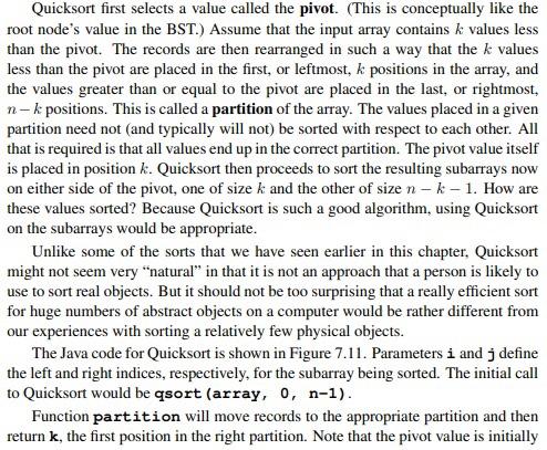
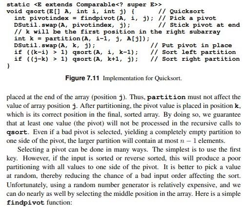
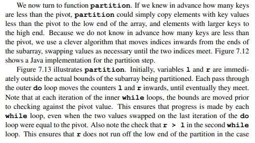
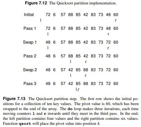
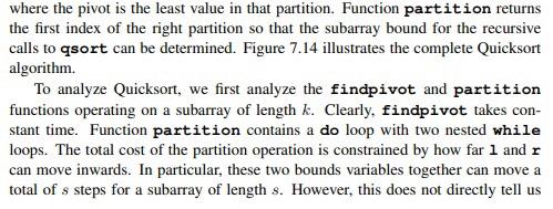
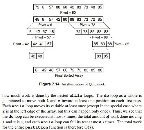
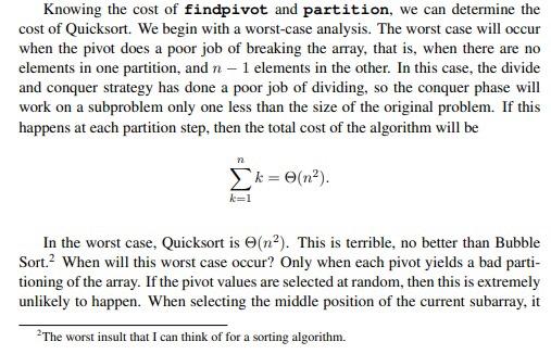
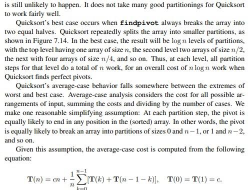
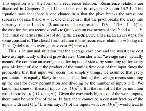
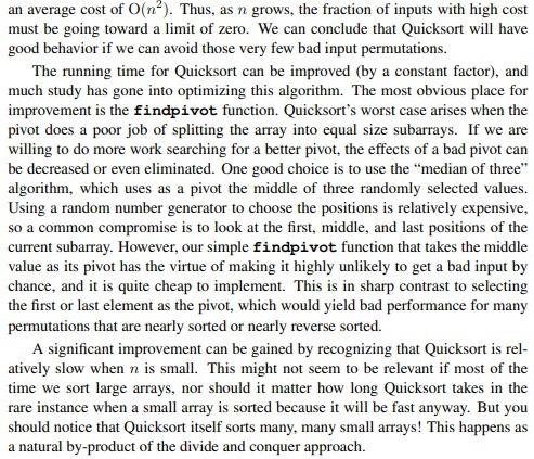
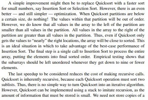
7.5 Quicksort While Mergesort uses the most obvious form of divide and conquer (split the list in half then sort the halves), it is not the only way that we can break down the sorting problem. And we saw that doing the merge step for Mergesort when using an array implementation is not so easy. So perhaps a different divide and conquer strategy might turn out to be more efficient? Quicksort is aptly named because, when properly implemented, it is the fastest known general-purpose in-memory sorting algorithm in the average case. It does not require the extra array needed by Mergesort, so it is space efficient as well. Quicksort is widely used, and is typically the algorithm implemented in a library sort routine such as the UNIX qsort function. Interestingly, Quicksort is ham- pered by exceedingly poor worst-case performance, thus making it inappropriate for certain applications. Before we get to Quicksort, consider for a moment the practicality of using a Binary Search Tree for sorting. You could insert all of the values to be sorted into the BST one by one, then traverse the completed tree using an inorder traversal. The output would form a sorted list. This approach has a number of drawbacks, including the extra space required by BST pointers and the amount of time required to insert nodes into the tree. However, this method introduces some interesting ideas. First, the root of the BST (i.e., the first node inserted) splits the list into two sublists: The left subtree contains those values in the list less than the root value while the right subtree contains those values in the list greater than or equal to the root value. Thus, the BST implicitly implements a "divide and conquer" approach to sorting the left and right subtrees. Quicksort implements this concept in a much more efficient way. Quicksort first selects a value called the pivot. (This is conceptually like the root node's value in the BST.) Assume that the input array contains k values less than the pivot. The records are then rearranged in such a way that the k values less than the pivot are placed in the first, or leftmost, k positions in the array, and the values greater than or equal to the pivot are placed in the last, or rightmost, n-k positions. This is called a partition of the array. The values placed in a given partition need not (and typically will not) be sorted with respect to each other. All that is required is that all values end up in the correct partition. The pivot value itself is placed in position k. Quicksort then proceeds to sort the resulting subarrays now on either side of the pivot, one of size k and the other of size n-k-1. How are these values sorted? Because Quicksort is such a good algorithm, using Quicksort on the subarrays would be appropriate. Unlike some of the sorts that we have seen earlier in this chapter, Quicksort might not seem very "natural" in that it is not an approach that a person is likely to use to sort real objects. But it should not be too surprising that a really efficient sort for huge numbers of abstract objects on a computer would be rather different from our experiences with sorting a relatively few physical objects. The Java code for Quicksort is shown in Figure 7.11. Parameters i and ; define the left and right indices, respectively, for the subarray being sorted. The initial call to Quicksort would be qsort (array, 0, n-1). Function partition will move records to the appropriate partition and then return k, the first position in the right partition. Note that the pivot value is initially static > void qsort (E[] a, int i, int i) { Il Quicksort int pivotindex = findpivot (A, i, j); // Pick a pivot DSutil.swap (A, pivotindex, j); // Stick pivot at end 1/ k will be the first position in the right subarray int k = partition (A, i-1, j, A[j]); DSutil.swap (A, k, 1); 1/ Put pivot in place if ((-i) > 1) qsort (A, i, k-1); // Sort left partition if ((j-k) > 1) qsort (A, k+1, j); // Sort right partition } Figure 7.11 Implementation for Quicksort. placed at the end of the array (position j). Thus, partition must not affect the value of array position j. After partitioning, the pivot value is placed in position k, which is its correct position in the final, sorted array. By doing so, we guarantee that at least one value (the pivot) will not be processed in the recursive calls to qsort. Even if a bad pivot is selected, yielding a completely empty partition to one side of the pivot, the larger partition will contain at most n - 1 elements. Selecting a pivot can be done in many ways. The simplest is to use the first key. However, if the input is sorted or reverse sorted, this will produce a poor partitioning with all values to one side of the pivot. It is better to pick a value at random, thereby reducing the chance of a bad input order affecting the sort. Unfortunately, using a random number generator is relatively expensive, and we can do nearly as well by selecting the middle position in the array. Here is a simple findpivot function: We now turn to function partition. If we knew in advance how many keys are less than the pivot, partition could simply copy elements with key values less than the pivot to the low end of the array, and elements with larger keys to the high end. Because we do not know in advance how many keys are less than the pivot, we use a clever algorithm that moves indices inwards from the ends of the subarray, swapping values as necessary until the two indices meet. Figure 7.12 shows a Java implementation for the partition step. Figure 7.13 illustrates partition. Initially, variables 1 and r are immedi- ately outside the actual bounds of the subarray being partitioned. Each pass through the outer do loop moves the counters 1 and r inwards, until eventually they meet. Note that at each iteration of the inner while loops, the bounds are moved prior to checking against the pivot value. This ensures that progress is made by each while loop, even when the two values swapped on the last iteration of the do loop were equal to the pivot. Also note the check that r > 1 in the second while loop. This ensures that r does not run off the low end of the partition in the case static > int partition (E[] A, int i, int r, E pivot) { do 1/ Move bounds inward until they meet while (A [++1].compareTo (pivot) 0)); DSutil.swap (A, 1, 1); 1/ Swap out-of-place values } while (1