Hello I need a MATLAB help, Am working on my Systems and Controls exercise where we are analyzing Open Loop Response of Dynamical Systems using ode45. We are suppose to create a function named second order for the main code to call. I am having trouble figuring it out and your help would be greatly appreciated in 1.1 & 1.2. I have copied the functions code at the bottom of the main code. I will attach the instructions and my code below, Thank you
NOTE: The values of A are as given.
function dy = second_order(t,y,u,a0,a1) A = [0 1; -2 -17]; B = [0 ; 1]; u = 1; dy = (A * y) + (B * u); end
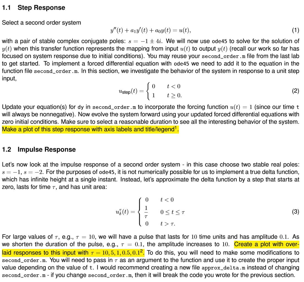
1.1 Step Response Select a second order system with a pair of stable complex conjugate poles: s =-14. We will now use ode45 to solve for the solution of y(t) when this transfer function represents the mapping from input u(t) to output y(t) (recall our work so far has focused on system response due to initial conditions). You may reuse your second_order.m file from the last lab to get started. To implement a forced differential equation with ode45 we need to add it to the equation in the function file second_order.m. In this section, we investigate the behavior of the system in response to a unit step input 0 t0 Update your equation(s) for dy in second_order .m to incorporate the forcing function u(t) (since our time t will always be nonnegative). Now evolve the system forward using your updated forced differential equations with zero initial conditions. Make sure to select a reasonable duration to see all the interesting behavior of the system Make a plot of this step response with axis labels and title/legend 1.2 Impulse Response Let's now look at the impulse response of a second order system in this case choose two stable real poles: s =-1, s =-2. For the purposes of ode45, it is not numerically possible for us to implement a true delta function, which has infinite height at a single instant. Instead, let's approximate the delta function by a step that starts at zero, lasts for time T, and has unit area: 0 tT. For large values of T, e.g., 10, we will have a pulse that lasts for 10 time units and has amplitude 0.1. As we shorten the duration of the pulse, e.g., 0.1, the amplitude increases to 10. Create a plot with over- laid responses to this input with T 10,5, 1, 0.5, 0.12. To do this, you will need to make some modifications to second-order, m. You will need to pass in as an argument to the function and use it to create the proper input value depending on the value of t. I would recommend creating a new file approx_delta.m instead of changing second order.m - if you change second_order.m, then it will break the code you wrote for the previous section. 1.1 Step Response Select a second order system with a pair of stable complex conjugate poles: s =-14. We will now use ode45 to solve for the solution of y(t) when this transfer function represents the mapping from input u(t) to output y(t) (recall our work so far has focused on system response due to initial conditions). You may reuse your second_order.m file from the last lab to get started. To implement a forced differential equation with ode45 we need to add it to the equation in the function file second_order.m. In this section, we investigate the behavior of the system in response to a unit step input 0 t0 Update your equation(s) for dy in second_order .m to incorporate the forcing function u(t) (since our time t will always be nonnegative). Now evolve the system forward using your updated forced differential equations with zero initial conditions. Make sure to select a reasonable duration to see all the interesting behavior of the system Make a plot of this step response with axis labels and title/legend 1.2 Impulse Response Let's now look at the impulse response of a second order system in this case choose two stable real poles: s =-1, s =-2. For the purposes of ode45, it is not numerically possible for us to implement a true delta function, which has infinite height at a single instant. Instead, let's approximate the delta function by a step that starts at zero, lasts for time T, and has unit area: 0 tT. For large values of T, e.g., 10, we will have a pulse that lasts for 10 time units and has amplitude 0.1. As we shorten the duration of the pulse, e.g., 0.1, the amplitude increases to 10. Create a plot with over- laid responses to this input with T 10,5, 1, 0.5, 0.12. To do this, you will need to make some modifications to second-order, m. You will need to pass in as an argument to the function and use it to create the proper input value depending on the value of t. I would recommend creating a new file approx_delta.m instead of changing second order.m - if you change second_order.m, then it will break the code you wrote for the previous