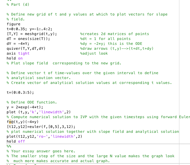
Hello, This is Matlab work. I am not very confident about my work.

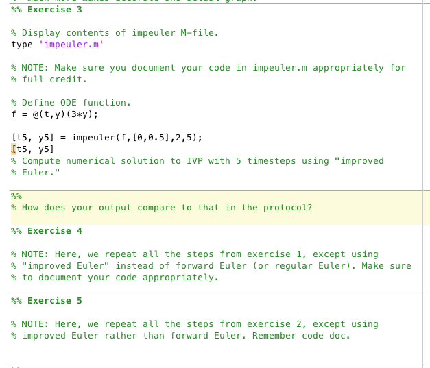
Could you check my work if they are correct, and I need help with 4&5.

I am lost at 4 & 5

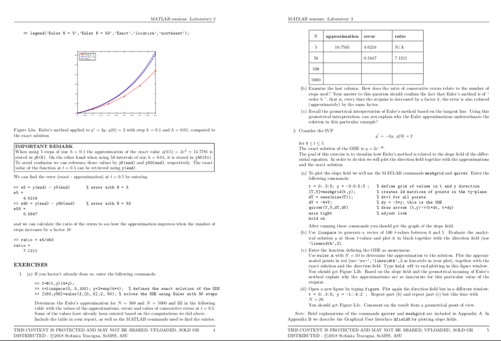
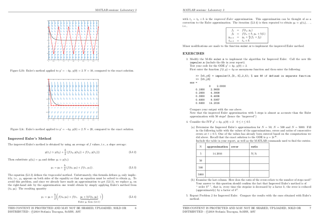
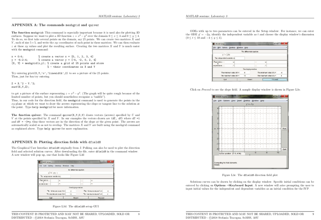
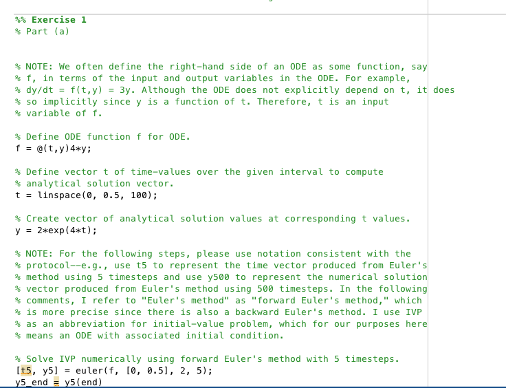
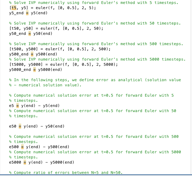
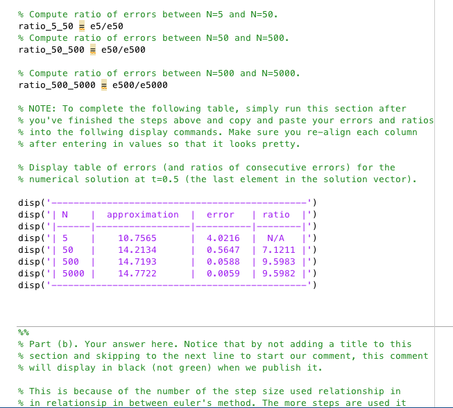
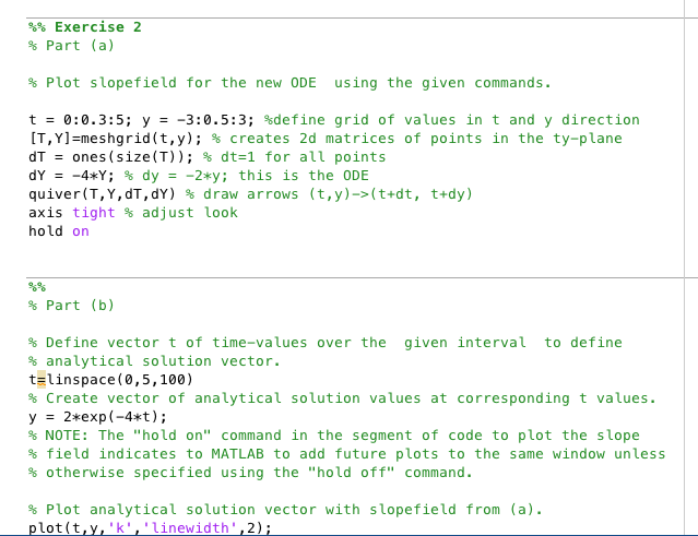
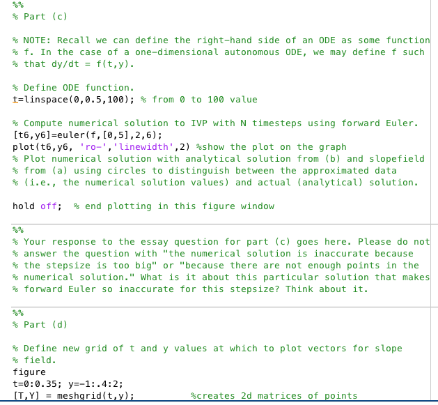
MATLAB ssos Laboratory 3 MATI.AB wskaas legead ('Euler N 5.Eler- 50. Exact.'locatioa' orthueat' N approximation error ratio N/A 7.1211 10 7565 .0216 0.5647 500 (b) Examine the lasto How does the rat io of osutive errors relate to the number o steps used? Your answer to this question should confirm the fact that Euler's method is of order h",that is, every time the stepsize is decreased by a factor k, the error is also reduced (approximately) by the e actor (c) Recall the geornetrical interpretation of Euler's method baued on the tangent line. Using this geometrical interpretation,can you explain why the Euler apprxinations underestimate the solution in this particular exmple? Figure L3a Euler's met hod applied to 4y, y(0)-2 with step h-0.1 and h-001, compared to t he exact solution 2Coider the IVP IMPORTANT REMARK When using 5 steps of siae0.1 the approxim at ion of the exact value 05) 214.7781 is stored in y (6). On the other hand when using 50 intervals of s h-001, it is stored in y50 (51) To avoid confusion we can reference these values by y5(end) and y50Cend), espect ively. The exact value of the function at t05 can be retrieved using y(end) The exact wolution of the ODE is y-2 The goal of this exrcise is to visualie how Euler's nethod is related to the slope field of the differ- ential equation In order to do this we will plot the direction field together with the approximations and the exact wolution (a) To plot the slope field we will the MATLAB commands neshgrid and qaiver. Enter the We can find the error (exact approximation) at t0.5 by entering following con mand t . 0: .3:5; y .-3:0.5:3 ; dT ones (aize CT) % error with N . 5 % define grid of values in t and y direction % createa 2d matrices of pointa in the ty-plane % d,.1 tor all points % dy .-3*y: this is the ODE 4.0216 >> e50 . y(end) -y50(end) 50 % error vith N . 50 quiver (T,Y,dT,dY axia tight hold on 0.5647 % adjust look and we can caleulate the rat io of the errons to see how the approximation impves when the number of steps increawes by a factor 10 After running these commands you sbould get the graph of the slope beld (b) Ue linspace to generate a wetor of 100 t-values between 0 and 5. Evaluate the analyt- > ratie5/e50 cal solution y at these t-values and plot it in black together with the dition feld (uw linevidth2) 7.1211 (c) Enter the function defining the ODE as anonymous. Use euler.n with N 10 to determine the approximation to the solution. Plot the appri- mated points in red rolinevidth',2 line-style in your plot),together with the exact solution and the direction field. Type hold off to end ploting in this figure window You shoukd get Figure LSb. Based on the slope field and the geomet rical meaning of Euler's method explain why the approcimations are so inaccurate for this part icular val ue of the stepsia EXERCISES L (a) If you haven't already done so, enter the following commands >> t"linapace(o, .5,100); y.2+exp (4et); % datinea the .xact olution of the ODE >> [tSo,y50].euler ce, [o,.5),2. 50); % aolven the ODE using Euler with 50 atepe (d) Open a new figure by typing igure. Plot again the direetion field bt in a different window t0:.3:5 y-1.4:2Repeat part (b) and reat part (c) but this time with N=20. You should get Figure L3e. Comment on the reault from a geometrical point of view Determine the Euler's approximation for N -500 and N- 5000 and fill in the Sollowing table with the values of the approxi mat ions, ers and ratios of consecutive errors at t0.S Sone of the values have already been entered based on the computations we did above. Include the table in your report, as well as the MATLAB commands used to find the entries Note: Brief explanat oas of the commands quiver and meahgrid are included in Appendix A. In Appedix B we describe the Geaphical Uwer Interace dfield8 for pktting skope fiekls THIS CONTENT IS PROTECTED AND MAY NOT BE SHARED, UPLOADED, SOLD OR DISTRIBUTED-92018 Stefania Tracogna, SoMSS, ASU THIS CONTENT IS PROTECTED AND MAY NOT BE SHARED, UPLOADED, SOLD OFR DISTRIBUTED-92018 Stefania Tracogna, SoMSS, ASU MATLAB ssos Laboratory 3 MATI.AB wskaas legead ('Euler N 5.Eler- 50. Exact.'locatioa' orthueat' N approximation error ratio N/A 7.1211 10 7565 .0216 0.5647 500 (b) Examine the lasto How does the rat io of osutive errors relate to the number o steps used? Your answer to this question should confirm the fact that Euler's method is of order h",that is, every time the stepsize is decreased by a factor k, the error is also reduced (approximately) by the e actor (c) Recall the geornetrical interpretation of Euler's method baued on the tangent line. Using this geometrical interpretation,can you explain why the Euler apprxinations underestimate the solution in this particular exmple? Figure L3a Euler's met hod applied to 4y, y(0)-2 with step h-0.1 and h-001, compared to t he exact solution 2Coider the IVP IMPORTANT REMARK When using 5 steps of siae0.1 the approxim at ion of the exact value 05) 214.7781 is stored in y (6). On the other hand when using 50 intervals of s h-001, it is stored in y50 (51) To avoid confusion we can reference these values by y5(end) and y50Cend), espect ively. The exact value of the function at t05 can be retrieved using y(end) The exact wolution of the ODE is y-2 The goal of this exrcise is to visualie how Euler's nethod is related to the slope field of the differ- ential equation In order to do this we will plot the direction field together with the approximations and the exact wolution (a) To plot the slope field we will the MATLAB commands neshgrid and qaiver. Enter the We can find the error (exact approximation) at t0.5 by entering following con mand t . 0: .3:5; y .-3:0.5:3 ; dT ones (aize CT) % error with N . 5 % define grid of values in t and y direction % createa 2d matrices of pointa in the ty-plane % d,.1 tor all points % dy .-3*y: this is the ODE 4.0216 >> e50 . y(end) -y50(end) 50 % error vith N . 50 quiver (T,Y,dT,dY axia tight hold on 0.5647 % adjust look and we can caleulate the rat io of the errons to see how the approximation impves when the number of steps increawes by a factor 10 After running these commands you sbould get the graph of the slope beld (b) Ue linspace to generate a wetor of 100 t-values between 0 and 5. Evaluate the analyt- > ratie5/e50 cal solution y at these t-values and plot it in black together with the dition feld (uw linevidth2) 7.1211 (c) Enter the function defining the ODE as anonymous. Use euler.n with N 10 to determine the approximation to the solution. Plot the appri- mated points in red rolinevidth',2 line-style in your plot),together with the exact solution and the direction field. Type hold off to end ploting in this figure window You shoukd get Figure LSb. Based on the slope field and the geomet rical meaning of Euler's method explain why the approcimations are so inaccurate for this part icular val ue of the stepsia EXERCISES L (a) If you haven't already done so, enter the following commands >> t"linapace(o, .5,100); y.2+exp (4et); % datinea the .xact olution of the ODE >> [tSo,y50].euler ce, [o,.5),2. 50); % aolven the ODE using Euler with 50 atepe (d) Open a new figure by typing igure. Plot again the direetion field bt in a different window t0:.3:5 y-1.4:2Repeat part (b) and reat part (c) but this time with N=20. You should get Figure L3e. Comment on the reault from a geometrical point of view Determine the Euler's approximation for N -500 and N- 5000 and fill in the Sollowing table with the values of the approxi mat ions, ers and ratios of consecutive errors at t0.S Sone of the values have already been entered based on the computations we did above. Include the table in your report, as well as the MATLAB commands used to find the entries Note: Brief explanat oas of the commands quiver and meahgrid are included in Appendix A. In Appedix B we describe the Geaphical Uwer Interace dfield8 for pktting skope fiekls THIS CONTENT IS PROTECTED AND MAY NOT BE SHARED, UPLOADED, SOLD OR DISTRIBUTED-92018 Stefania Tracogna, SoMSS, ASU THIS CONTENT IS PROTECTED AND MAY NOT BE SHARED, UPLOADED, SOLD OFR DISTRIBUTED-92018 Stefania Tracogna, SoMSS, ASU