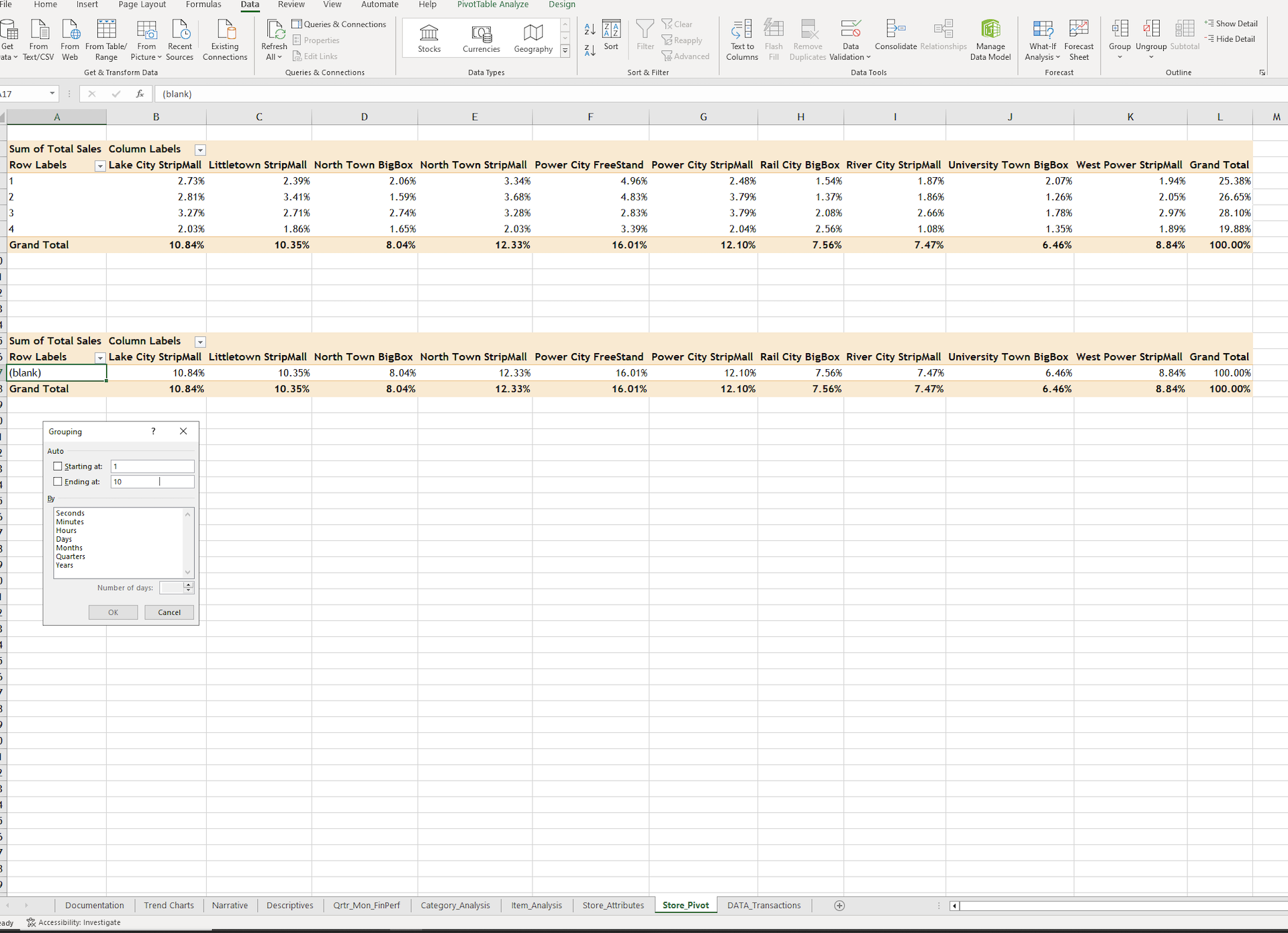
I am currently working on part 8.

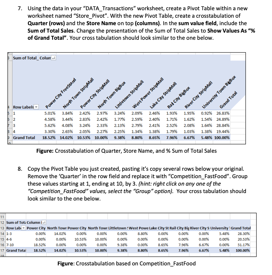
This is what I am trying to accomplish. I am having trouble grouping it as the example shows. This on excel.

This is what comes up when I try to accomplish it.

7. Using the data in your "DATA_Transactions" worksheet, create a Pivot Table within a new worksheet named "Store_Pivot". With the new Pivot Table, create a crosstabulation of Quarter (rows) and the Store Name on top (columns). In the sum value field, include the Sum of Total Sales. Change the presentation of the Sum of Total Sales to Show Values As "\% of Grand Total". Your cross tabulation should look similar to the one below. Figure: Crosstabulation of Quarter, Store Name, and \% Sum of Total Sales 8. Copy the Pivot Table you just created, pasting it's copy several rows below your original. Remove the 'Quarter' in the row field and replace it with "Competition_FastFood". Group these values starting at 1 , ending at 10 , by 3 . (hint: right click on any one of the "Competition_FastFood" values, select the "Group" option). Your cross tabulation should look similar to the one below. Figure: Crosstabulation based on Competition_FastFood