I need some help with the Question (3) of this MATLAB assignment, I try to run my code but it keeps giving me error, please help me to correct it, thank you!

here's the details about this assignment

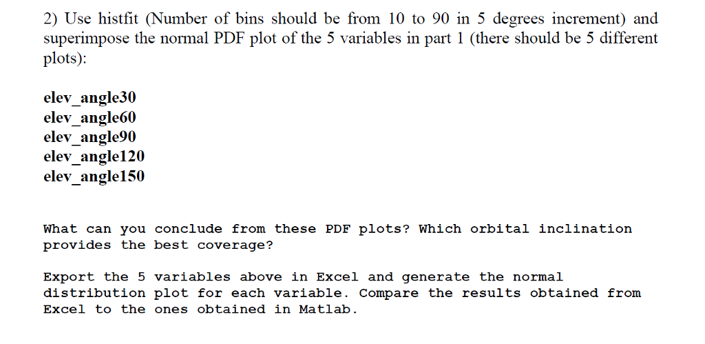
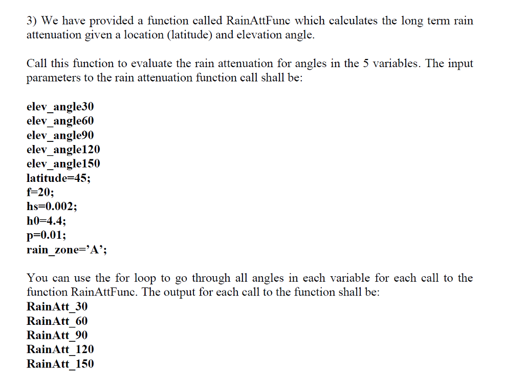
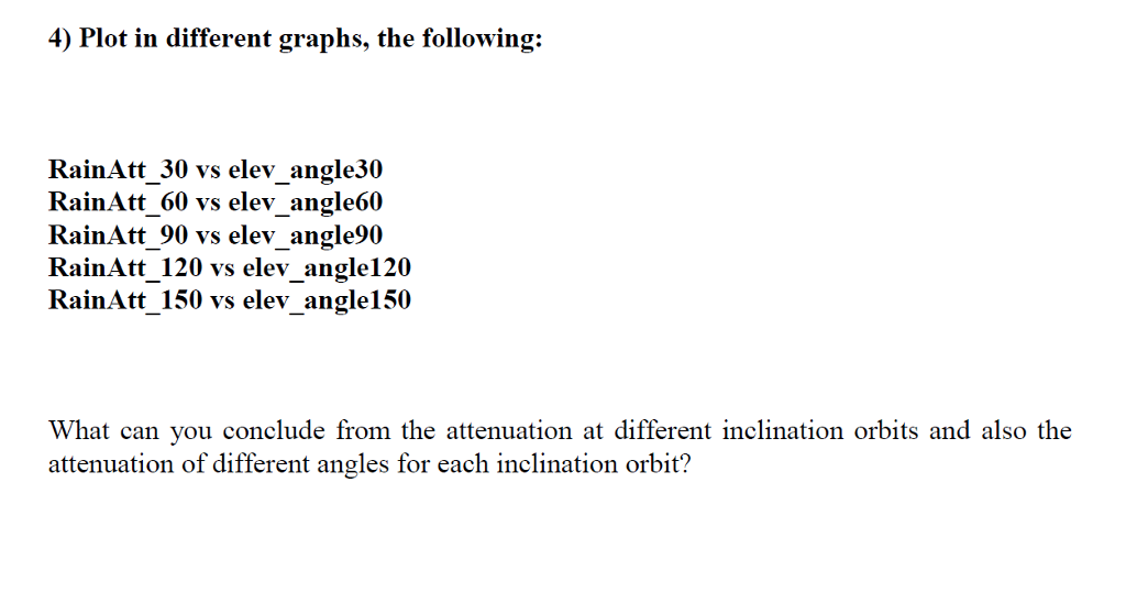
the documents

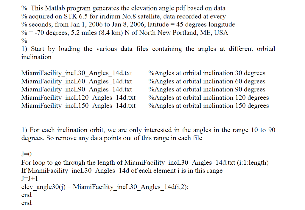
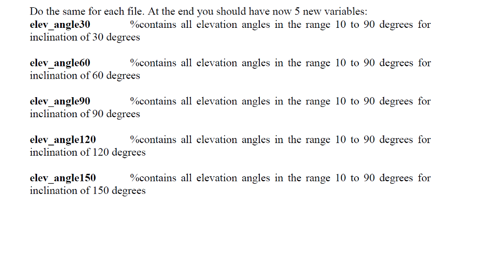
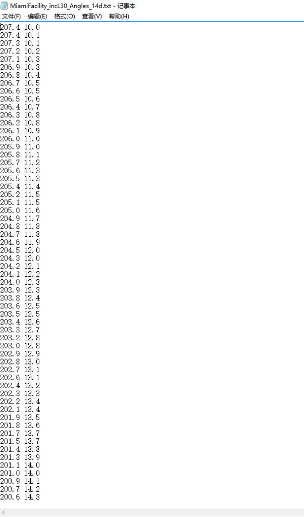
MiamiFacility_incL30_Angles_14d.txt MiamiFacility_incL60_Angles_14d.txt MiamiFacility_incL90_Angles_14d.txt MiamiFacility_incL120_Angles_14d.txt MiamiFacility_incL150_Angles_14d.txt

they are lists contains datas like the graph below

And here is function RainAttFunc which is given by the instructor

function [Ap] = RainAttFunc(p, rain_zone, hs, theta, latitude, f, h0)

% Rp: point rainfall rate for the location for a chosen percentage of time of % an average year (mm/h) % Define rain climatic zones (Table 1) from ITU-R PN.837-1 for p=0.01% R001 = [8 12 15 19 22 28 30 32 35 42 60 63 95 145 115];

% Get percentage of time in % %p = input('Enter the Percentage of Time (%):');

% Get rain climatic zone from user input %rain_zone = input('Enter the Rain Zone(capitalized):' , 's'); if rain_zone == 'A' col_chosen = 1;

elseif rain_zone == 'B' col_chosen = 2; elseif rain_zone == 'C' col_chosen = 3; elseif rain_zone == 'D' col_chosen = 4;

elseif rain_zone == 'E' col_chosen = 5;

elseif rain_zone == 'F' col_chosen = 6; elseif rain_zone == 'G' col_chosen = 7; elseif rain_zone == 'H' col_chosen = 8; elseif rain_zone == 'J' col_chosen = 9; elseif rain_zone == 'K' col_chosen = 10; elseif rain_zone == 'L' col_chosen = 11; elseif rain_zone == 'M' col_chosen = 12; elseif rain_zone == 'N' col_chosen = 13; elseif rain_zone == 'P' col_chosen = 14; elseif rain_zone == 'Q' col_chosen = 15; else col_chosen = 0; end

% hs: height above mean sea level of the earth station (km) % If not sure about this, we ASSUME it is equal to zero %hs = input('Enter the height above mean sea level of the earth station (km):'); if isempty(hs) hs = 0; end

% theta: elevation angle (degrees) %theta = input('Enter the elevation angle (degrees):');

% latitude: latitude of the earth station (degrees) %latitude = input('Enter the latitude of the earth station (degrees):');

% f: frequency (GHz) %f = input('Enter the frequency (GHz):');

% Re: effective radius of the Earth (8500 km) Re = 8500;

% h0: 0'C isotherm height above mean sea level(km) %h0 = input('Enter the isotherm height (from Figure 1 of ITU-R P.839-3):');

% step 1: determine rain height, hR (from ITU-R P.839) hR = h0 + 0.36;

% Note: if hR-hs is less than or equal to zero, the predicted rain attenuation(Ap) is % zero, and the following steps are not required if (hR-hs

% step 2: compute slant-path length, Ls (km) if theta >= 5 Ls = (hR - hs)/ sin(theta/180*pi); else Ls = 2*(hR-hs)/(sqrt((sin(theta/180*pi))^2 + 2*(hR-hs)/Re) + sin(theta/180*pi)); end

% step 3: calculate the horizontal projection, LG (km) LG = Ls*cos(theta/180*pi); % step 4: obtain rainfall rate (R001 defined earlier), here based on p = 0.01%

% step 5: obtain the specific attenuation, gamaR (from ITU-R P.838) % Note: in order to make the program work with all frequencies from 1 to % 1000 GHz, instead of using existing results in Table 5, we go through the % derivation of k and alfa

% load coefficients table,(i, j), i:1=table1,2=table2,3=table3,4=table4 load('a.txt'); load('b.txt'); load('c.txt');

% for kH first_term = 0; for j = 1:1:4 first_term = first_term + a(1,j)*exp(-((log(f)/log(10) - b(1,j))/c(1,j))^2); end second_term = -0.18961*log(f)/log(10) + 0.71147; kH = 10^(first_term + second_term);

% for kV first_term = 0; for j = 1:1:4 first_term = first_term + a(2,j)*exp(-((log(f)/log(10) - b(2,j))/c(2,j))^2); end second_term = -0.16398*log(f)/log(10) + 0.63297; kV = 10^(first_term + second_term);

% for alfaH first_term = 0; for j = 1:1:5 first_term = first_term + a(3,j)*exp(-((log(f)/log(10) - b(3,j))/c(3,j))^2); end second_term = 0.67849*log(f)/log(10) - 1.95537; alfaH = (first_term + second_term);

% for alfaV first_term = 0; for j = 1:1:5 first_term = first_term + a(4,j)*exp(-((log(f)/log(10) - b(4,j))/c(4,j))^2); end second_term = -0.053739*log(f)/log(10) + 0.83433; alfaV = (first_term + second_term);

% now, use equation (2) and (3) to find out values for k and alfa % Note: here, we ASSUME delta = 45 degrees for circular polarization delta = 45; k = (kH + kV + (kH-kV)*((cos(theta/180*pi))^2)*cos(2*delta/180*pi))/2; alfa = (kH*alfaH + kV*alfaV + (kH*alfaH - kV*alfaV)*((cos(theta/180*pi))^2)*cos(2*delta/180*pi))/(2*k);

% finally, gamaR (dBm/km): gamaR = k*(R001(col_chosen))^alfa;

% step 6: calculate the horizontal reduction factor, rp rp = 1/(1+0.78*sqrt((LG*gamaR)/f)-0.38*(1-exp(-2*LG)));

% step 7: calculate the vertical adjustment factor, vp phi = atan((hR-hs)/(LG*rp));

if (phi/pi*180) > theta LR = (LG*rp)/cos(theta/180*pi); else LR = (hR-hs)/sin(theta/180*pi); end

if (latitude

vp = 1/(1+sqrt(sin(theta/180*pi))*(31*(1-exp(-(theta/(1+x)))*(sqrt(LR*gamaR))/(f^2))-0.45));

% step 8: compute the effective path length, LE LE = LR*vp;

% step 9: the predicted attenuation exceeded for 0.01% is (dB): % Note: this is for p = 0.01% Ap01 = gamaR*LE;

% step 10: for other p values from 0.001% to 5% if (p>=1) || (abs(latitude)>=36) beta = 0; elseif (p=25) beta = -0.005*(abs(latitude)-36); else beta = -0.005*(abs(latitude)-36)+1.8-4.25*sin(theta/180*pi); end

% final estimated attenuation (Ap) for 0.01% or others if(p == 0.01) Ap = Ap01; else Ap = Ap01*(p/0.01)^(-(0.655+0.0331*log(p)-0.045*log(Ap01)-beta*(1-p)*sin(theta/180*pi))); end

and here is my work

%%% Q1 %%% %% %%% elev_angle30 %%% clear A=dlmread('MiamiFacility_incL30_Angles_14d.txt'); La=length(A);

j=0;

for i=1:La if A(i) >=10 && A(i)

%%% elev_angle60 %%%

B=dlmread('MiamiFacility_incL60_Angles_14d.txt'); Lb=length(B);

j=0;

for i=1:Lb if B(i) >=10 && B(i)

%%% elev_angle90 %%%

C=dlmread('MiamiFacility_incL90_Angles_14d.txt'); Lc=length(C);

j=0;

for i=1:Lc if C(i) >=10 && C(i)

%%% elev_angle120 %%%

D=dlmread('MiamiFacility_incL120_Angles_14d.txt'); Ld=length(D);

j=0;

for i=1:Ld if D(i) >=10 && D(i)

%%% elev_angle150 %%%

E=dlmread('MiamiFacility_incL150_Angles_14d.txt'); Le=length(E);

j=0;

for i=1:Le if E(i) >=10 && E(i)

%%% Q2 %%%

figure histfit(elev_angle30);

figure histfit(elev_angle60);

figure histfit(elev_angle90);

figure histfit(elev_angle120);

figure histfit(elev_angle150);

xlswrite('Assi30.xlsx',elev_angle30); xlswrite('Assi60.xlsx',elev_angle60); xlswrite('Assi90.xlsx',elev_angle90); xlswrite('Assi120.xlsx',elev_angle120); xlswrite('Assi150.xlsx',elev_angle150);

%%% Q3 %%%

latitude=45; f=20; hs=0.002; h0=4.4; p=0.01; rain_zone='A';

for t=1:La RainAtt_30(t) = RainAttFunc(p, rain_zone, hs,elev_angle30(t) , latitude, f, h0); end histfit(RainAtt_30); for t=1:Lb RainAtt_60(t)= RainAttFunc(p, rain_zone, hs, elev_angle60(t), latitude, f, h0); end

for t=1:Lc RainAtt_90(t)= RainAttFunc(p, rain_zone, hs, elev_angle90(t), latitude, f, h0); end

for t=1:Ld RainAtt_120(t)= RainAttFunc(p, rain_zone, hs, elev_angle120(t), latitude, f, h0); end

for t=1:Le RainAtt_15(t)= RainAttFunc(p, rain_zone, hs, elev_angle150(t), latitude, f, h0); end %%%%%%%%%%%% 30 degree from zone B to zone Q %%%%%%%%%%%%%%% t30=1; for rain_zone='B':'Q' for t=1:La RainAtt_30(t30) = RainAttFunc(p, rain_zone, hs,elev_angle30(t) , latitude, f, h0); t30=t30+1; end t30=t30+La-1; end histfit(RainAtt_30); histfit(elev_angle30); %%% Q4 %%%

%%%%%%%%%%%%%%%%%%%%% RainAtt_30 vs elev_angle30 figure histfit(RainAtt_30) hold on; histfit(elev_angle30) hold off; %%%%%%%%%%%%%%%%%%%%% RainAtt_60 vs elev_angle60 figure histfit(RainAtt_60) hold on; histfit(elev_angle60) hold off; %%%%%%%%%%%%%%%%%%%%% RainAtt_90 vs elev_angle90 figure histfit(RainAtt_90) hold on; histfit(elev_angle90) hold off; %%%%%%%%%%%%%%%%%%%%% RainAtt_120 vs elev_angle120 figure histfit(RainAtt_120) hold on; histfit(elev_angle120) hold off; %%%%%%%%%%%%%%%%%%%%% RainAtt_150 vs elev_angle150 figure histfit(RainAtt_150) hold on; histfit(elev_angle150) hold off;

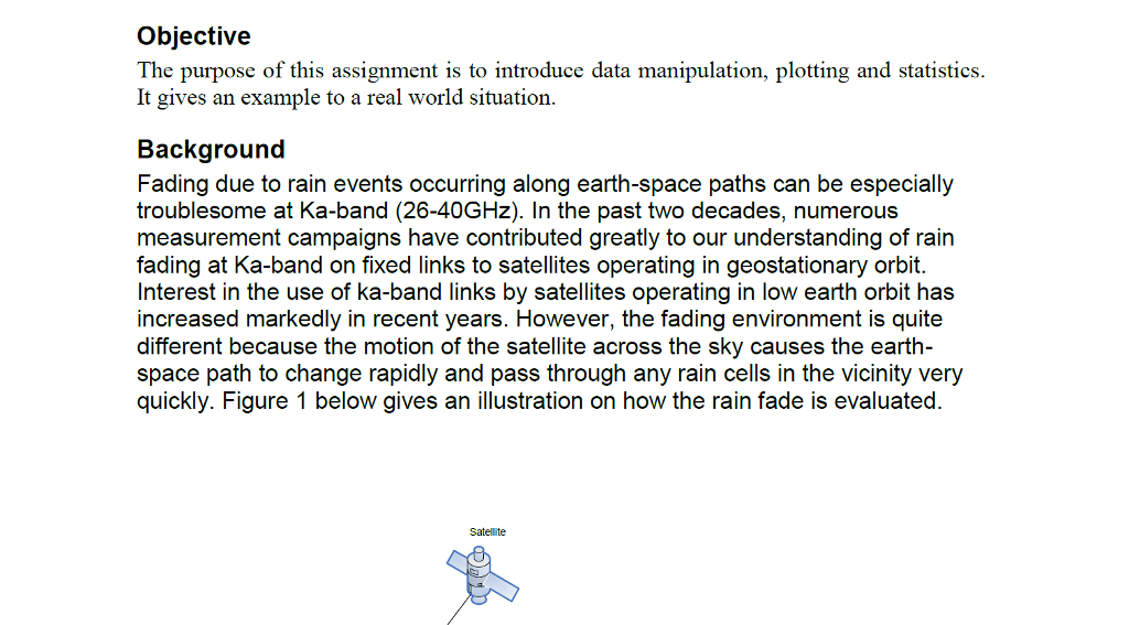
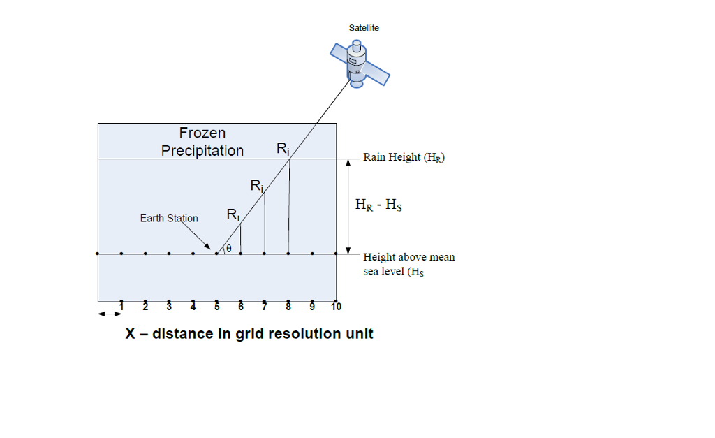
Objective The purpose of this assignment is to introduce data manipulation, plotting and statistics It gives an example to a real world situation. Background Fading due to rain events occurring along earth-space paths can be especially troublesome at Ka-band (26-40GHz). In the past two decades, numerous measurement campaigns have contributed greatly to our understanding of rain fading at Ka-band on fixed links to satellites operating in geostationary orbit. Interest in the use of ka-band links by satellites operating in low earth orbit has increased markedly in recent years. However, the fading environment is quite different because the motion of the satellite across the sky causes the earth- space path to change rapidly and pass through any rain cells in the vicinity very quickly. Figure 1 below gives an illustration on how the rain fade is evaluated. Satellite