i need your help please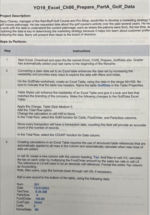

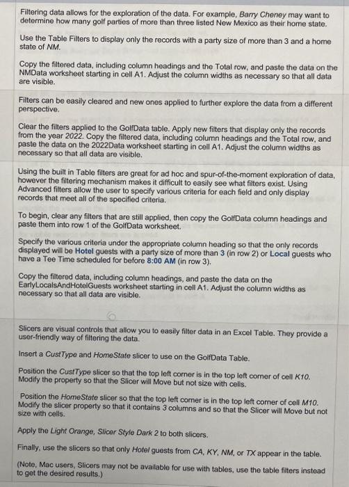
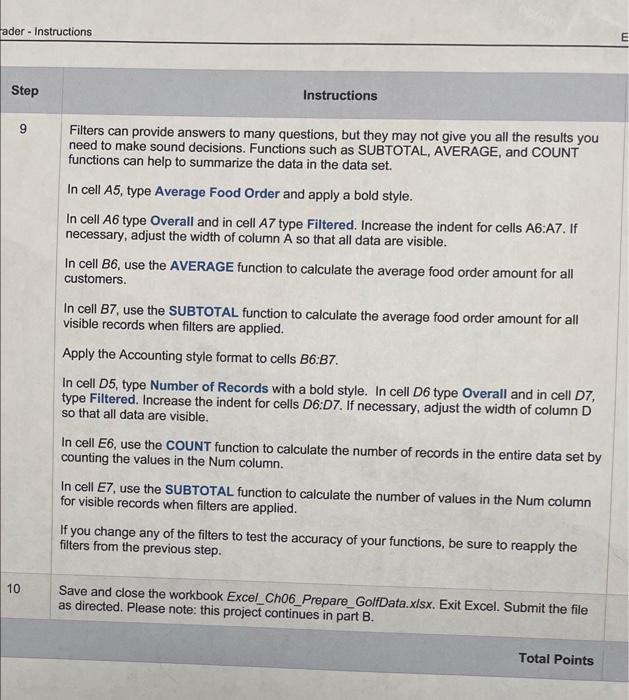
YO19_Excel_Ch06_Prepare_PartA_Golf_Data Project Description: Barry Cheney, manager of the Red Bluff Golf Course and Pro Shop, would like to develop a marketing strategy f olf course patronago. He has requested data about the golf course's activity over the past several years. He ne o work with the data to understand the current patronage, such as where the patrons were from, the tee time, an Exploring the data is key in determining the marketing strategy because it helps him leam about customer prefor inalyzing the data, Barry will present their ideas to the board of directors. Steps to Perform: Step Instructions Start Excel. Download and open the file named Excel_Ch06_Prepare_GoltData.xlsx. Grader has automatically added your last name to the beginning of the filename. 2 Converting a plain data set to an Excel table enhances the data set by increasing the readability and provides easy ways to explore the data with filters and totals. On the GolfDato worksheet, create an Excel Table, using the dato in the range A9:H39. Be sure to indicate that the table has headers. Name the table GoliData in the Table Properties. 3 Table Styles can enhance the readability of an Excel Table and give it a look and feel that matches the branding of the company. Make the following changes to the GollData Excel Table: Apply the Orange. Table Style Medium 3. Add the Total Row option. Change the calculation in cell H4O to None. In the Total Row, select the SUM function for Carts, FoodOrder, and PartySize columns. Since every transaction will have a transaction date, counting this field will provide an accurate count of the number of records. In the Total Row, select the COUNT function for Date column. Creating calculations in an Excel Table requires the use of structured table references that are automatically applied to all rows in the column and automatically calculate when new rows of data are added. In cell 19, create a new column with the column heading. Tax. And then in cell 110 , calculate the tax on each order by mukiplying the FoodOrder amount by the sales tax rate in cell L9. The reference to 9 will need to be an absolute cell reference. Format the entire Tax column as Accounting. Note, Mac users, copy the formula down through cell 139, if necessary. Add a new record to the bottom of the table, using the following data: NumDateTeeTimePartySizeFoodOrderCustTypeCartsHomeState20112/31/20228:30AM4104.80Hotel2WI Filtering data allows for the exploration of the data. For example, Barry Cheney may want to determine how many golf parties of more than three listed New Mexico as their home state. Use the Table Filters to display only the records with a party size of more than 3 and a home state of NM. Copy the filtered data, including column headings and the Total row, and paste the data on the NMData worksheet starting in cell A1. Adjust the column widths as necessary so that all data are visible. Filters can be easily cleared and new ones applied to further explore the data from a different perspective. Clear the filters applied to the GolfData table. Apply new filters that display only the records from the year 2022. Copy the filtered data, including column headings and the Total row, and paste the data on the 2022Data worksheet starting in coll A1. Adjust the column widths as necessary so that all data are visible. Using the built in Table filters are great for ad hoc and spur-of-the-moment exploration of data, however the fittering mechanism makes it difficult to easily see what filters exist. Using Advanced filters allow the user to specify various criteria for each field and only display records that meet all of the specified criteria. To begin, clear any filters that are still applied, then copy the GolfData column headings and paste them into row 1 of the GolfData worksheet. Specify the various criteria under the appropriate column heading so that the only records displayed will be Hotel guests with a party size of more than 3 (in row 2) or Local guests who have a Tee Time scheduled for before 8:00 AM (in row 3). Copy the fittered data, including column headings, and paste the data on the EarlyLocalsAndHotelGuests worksheet starting in cell A1. Adjust the column widths as necessary so that all data are visible. Slicers are visual controls that allow you to easily filter data in an Excel Table. They provide a user-friendly way of filtering the data. Insert a CustType and HomeState slicer to use on the GolfData Table. Position the CustType slicer so that the top left corner is in the top left comer of cell KTO. Modify the property so that the Slicer will Move but not size with cells. Position the HomeState slicer so that the top left comer is in the top left corner of cell M10. Modify the slicer property so that it contains 3 columns and so that the Slicer will Move but not size with cells. Apply the Light Orange, Slicer Style Dark 2 to both slicers. Finally, use the slicers so that only Hotel guests from CA,KY,NM, or TX appear in the table. (Note, Mac users, Slicers may not be available for use with tables, use the table filters instead to get the desired results.) Filters can provide answers to many questions, but they may not give you all the results you need to make sound decisions. Functions such as SUBTOTAL, AVERAGE, and COUNT functions can help to summarize the data in the data set. In cell A5, type Average Food Order and apply a bold style. In cell A6 type Overall and in cell A7 type Filtered. Increase the indent for cells A6:A7. If necessary, adjust the width of column A so that all data are visible. In cell B6, use the AVERAGE function to calculate the average food order amount for all customers. In cell B7, use the SUBTOTAL function to calculate the average food order amount for all visible records when filters are applied. Apply the Accounting style format to cells B6:B7. In cell D5, type Number of Records with a bold style. In cell D6 type Overall and in cell D7, type Filtered. Increase the indent for cells D6:D7. If necessary, adjust the width of column D so that all data are visible. In cell E6, use the COUNT function to calculate the number of records in the entire data set by counting the values in the Num column. In cell E7, use the SUBTOTAL function to calculate the number of values in the Num column for visible records when filters are applied. If you change any of the filters to test the accuracy of your functions, be sure to reapply the filters from the previous step. Save and close the workbook Excel_Ch06_Prepare_GolfData.x/sx. Exit Excel. Submit the file as directed. Please note: this project continues in part B