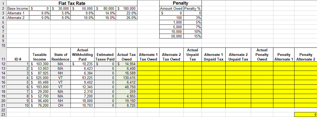
In cell G12, write a formula to calculate the total tax amount for Alternate 1 on the income in cell B12. Use the HLOOKUP function to determine the Alternate 1 flat tax rate for the income in cell B12 and then multiply by the income to get the dollar amount owed. If done properly the result in G12 should be 14,462.

Make sure you have used absolute references appropriately and then autofill down.

In cell H12, write a formula to calculate the total tax amount for alternate 2 on the income in cell B12. Use the HLOOKUP function to determine the Alternate 2 flat tax rate for the income in cell B12 and then multiply by the income to get the dollar amount owed. If done properly the result in H12 should be 16,528.

Make sure you have used absolute references appropriately and then autofill down.

In cell I12, write a formula to calculate the amount of unpaid taxes based on the Actual Tax Owed (column F) and the Actual Withholding Paid (column D). This is simply the difference between column F and column D. If done properly the result in I12 should be 4,719. Autofill down.

In cell J12, write a formula to calculate the amount of unpaid taxes based on the Alternate 1 Tax Owed (column G) and the Actual Withholding Paid (column D). This is simply the difference between column G and column D. If done properly the result in J12 should be 4,227. Autofill down.

In cell K12, write a formula to calculate the amount of unpaid taxes based on the Alternate 2 Tax Owed (column H) and the Actual Withholding Paid (column D). This is simply the difference between column H and column D. If done properly the result in K12 should be 6,293. Autofill down.

In cell L12, write a formula to calculate the Actual penalty owed IF the Actual unpaid tax in I12 is >0. You can LOOKUP the penalty rate in cells H3:I8. You will need to use IF, VLOOKUP and then multiplication. If done properly the result in L12 should be 236.

If necessary, modify your original formula in cell L12 with the appropriate absolute references so that you could have copied it across to column M and N and down to row 21.

Flat Tax Rate Penalty 2 Base Income S 3 Alternate 1 0 30,00050000 Amount Owed Penalty % 9 0% 1. 14 0% 16.0% 5 0% 22 0% 0.0% 0.0% Alternate 2 100 1,000 5,000 10,000 50,000 3% 5% 7% 10% 15% 10 Actual Actual Actual TaxableState of Withholding Estimated Actual Tax Alternate 1 Alternate 2Unpaid AlternateAlternate 2 Penalty Penalty Penalty Income Residence Paid Taxes PaidOwed Tax OwedTax Owed Tax Unpaid Tax Unpaid Tax Owed Alternate 1 Alternate 2 MA0,235 S 12 13 14 15 16 17 18 0 14.954 2S53,003 3 S 87,925 6,423 6,384 93,225 6,400 16,589 VT 6,412 12,345 2,310 7,200 18,000 10,703 7 S 29,200 8 S 52,700 9 $ 96,400 10S 76.200 259 4,955 19,192 ,725 ?!?2.fut) NA 20 21 NH 23