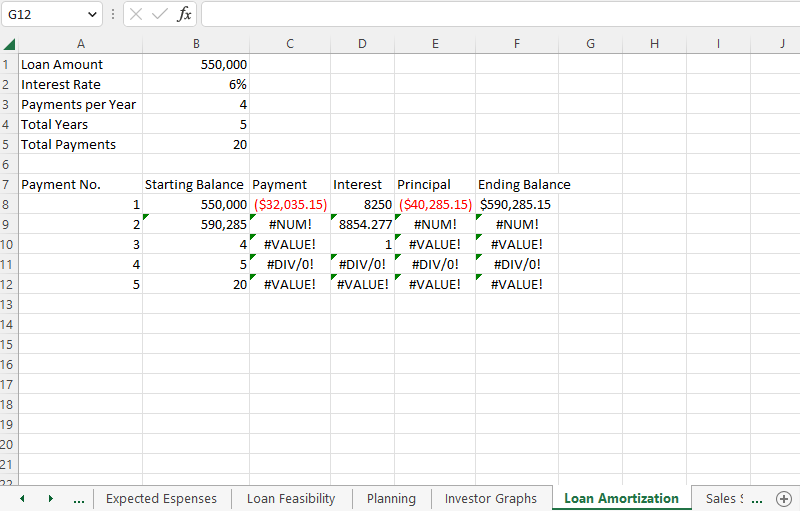
In Excel, I need help with this, please. I have the worksheet created but it is not adding up correctly. Please look at the screenshots provided. THANKS

Loan Amortization Schedule Worksheet

1. Create a new worksheet and name this new sheet to Loan Amortization.
2. In cell A1, type Loan Amount and in cell B1, enter $550,000.
3. In cell A2, type Interest Rate and in cell B2, enter 6%.
4. In cell A3, type Payments per Year and in cell B3, enter 4 (for quarterly payments).
5. In cell A4, type Total Years and in cell B4, enter 5.
6. In cell A5, type Total Payments.
7. In cell B5, enter the formula =B3 * B4.
8. Add the table headers
   • In cell A7, type Payment No.
   • In cell B7, type Starting Balance
   • In cell C7, type Payment
   • In cell D7, type Interest
   • In cell E7, type Principal
   • In cell F7, type Ending Balance
9. In cell A8, type 1.
10. In cell B8, enter =B1 (this refers back to your initial loan amount).
11. In cell C8, enter the PMT formula: =PMT(B2/B3, B5, B1). This will calculate the quarterly payment.
12. In cell D8, enter the formula =B8 * (B2/B3) to calculate the interest portion of the first payment.
13. In cell E8, enter the formula =C8 - D8 to calculate the principal portion of the first payment.
14. In cell F8, enter the formula =B8 - E8 to find the ending balance after the first payment.
15. Highlight cells A8 to F8. Drag the fill handle (small square at the bottom-right of the selection) down until you reach the row corresponding to your last payment (as per B5).
16. In the Starting Balance column (B), starting from cell B9, replace the formula with =F8 (the ending balance from the previous payment).
17. In the Interest column (D), starting from cell D9, replace the formula with =B9 * (B2/B3).
18. In the Principal column (E), starting from cell E9, replace the formula with =C9 - D9.
19. In the Ending Balance column (F), starting from cell F9, replace the formula with =B9 - E9.

G12 fx \begin{tabular}{|c|c|c|c|c|c|c|c|c|c|} \hline 4 & A & B & C & D & E & F & G & H & 1 \\ \hline & Loan Amount & 550,000 & & & & & & & \\ \hline & Interest Rate & 6% & & & & & & & \\ \hline & Payments per Year & 4 & & & & & & & \\ \hline & Total Years & 5 & & & & & & & \\ \hline & Total Payments & 20 & & & & & & & \\ \hline & & & & & & & & & \\ \hline & Payment No. & Starting Balance & Payment & Interest & Principal & Ending Balance & & & \\ \hline & 1 & 550,000 & ($32,035.15) & 8250 & ($40,285.15) & $590,285.15 & & & \\ \hline & 2 & 590,285 & \#NUM! & 8854.277 & \#NUM! & \#NUM! & & & \\ \hline & 3 & 4 & \#VALue! & 1 & \#VALUe! & \#VALUE! & & & \\ \hline & 4 & 5 & \#DIV/0! & \#DIV/0! & \#DIV/0! & \#DIV/0! & & & \\ \hline & 5 & 20 & \#VALUE! & \#VALUE! & \#VALUe! & \#VAlue! & & & \\ \hline & & & & & & & & & \\ \hline & & & & & & & & & \\ \hline & & & & & & & & & \\ \hline & & & & & & & & & \\ \hline & & & & & & & & & \\ \hline & & & & & & & & & \\ \hline & & & & & & & & & \\ \hline & & & & & & & & & \\ \hline & & & & & & & & & \\ \hline \end{tabular}