JAVA OR C

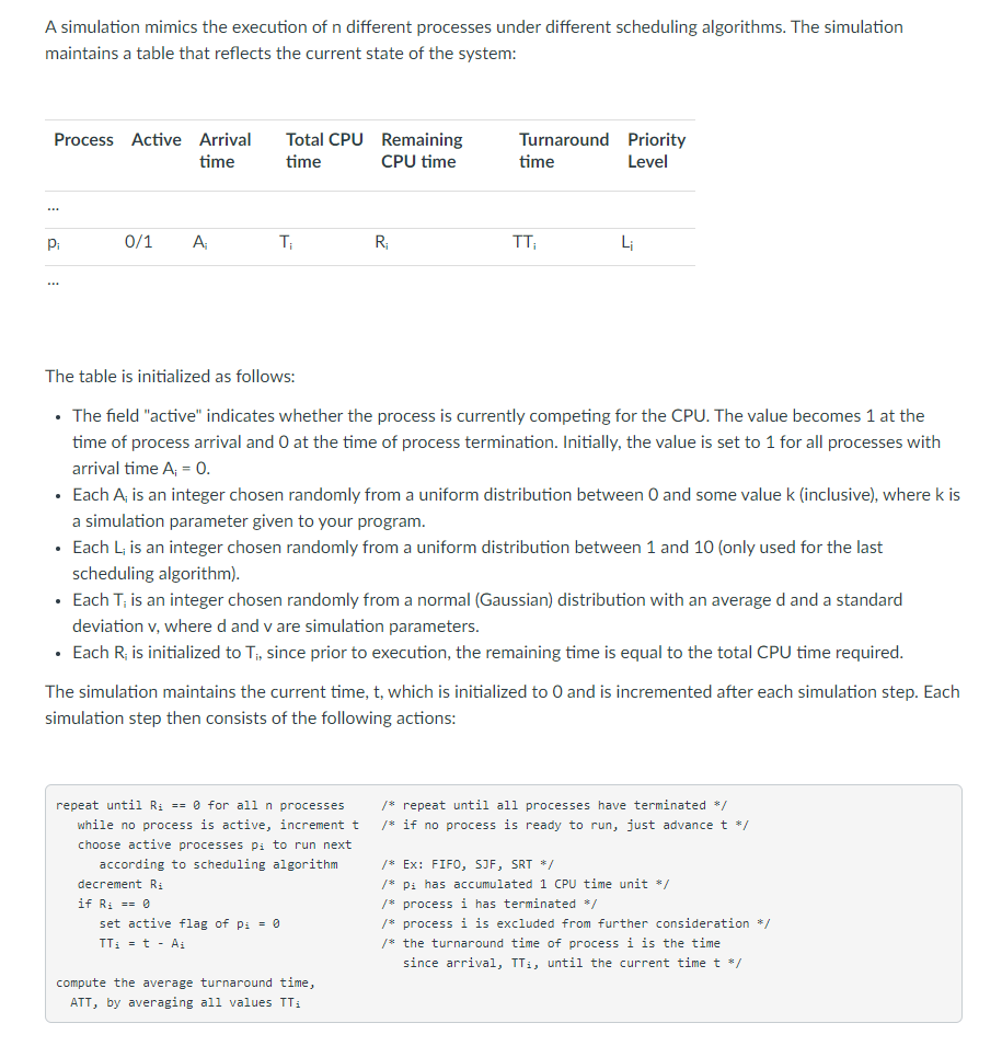
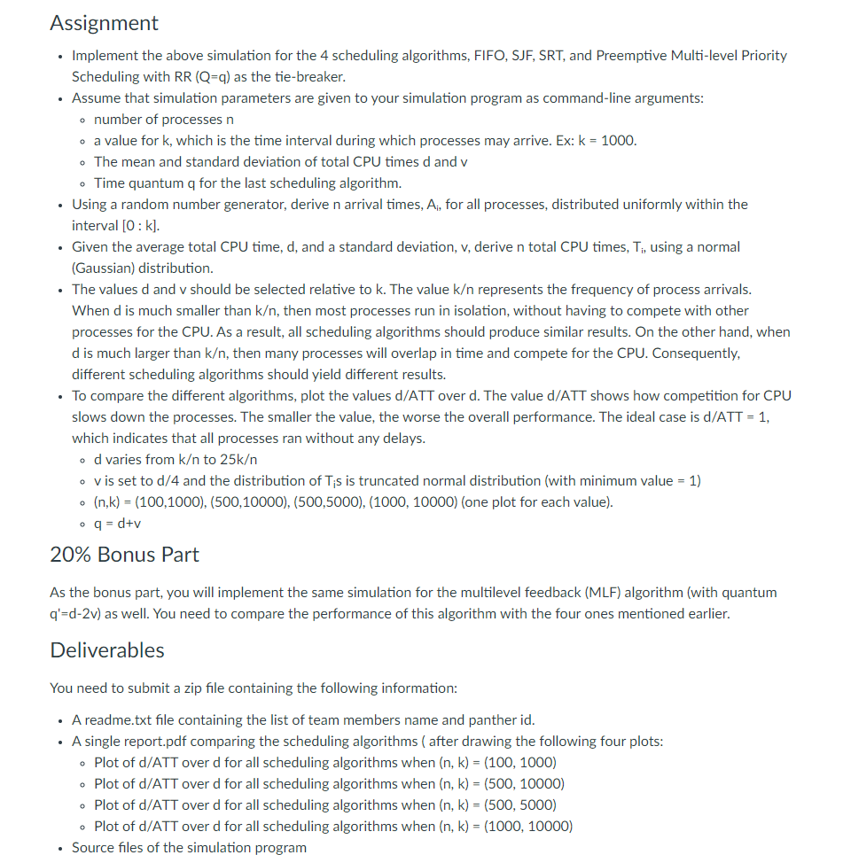
A simulation mimics the execution of n different processes under different scheduling algorithms. The simulation maintains a table that reflects the current state of the system: Process Active Arrival time Total CPU Remaining time CPU time Turnaround Priority time Level P 0/1 . TE R; TT: Li The table is initialized as follows: The field "active" indicates whether the process is currently competing for the CPU. The value becomes 1 at the time of process arrival and 0 at the time of process termination. Initially, the value is set to 1 for all processes with arrival time A; = 0. Each A; is an integer chosen randomly from a uniform distribution between 0 and some value k (inclusive), where k is a simulation parameter given to your program. Each L; is an integer chosen randomly from a uniform distribution between 1 and 10 (only used for the last scheduling algorithm). Each T; is an integer chosen randomly from a normal (Gaussian) distribution with an average d and a standard deviation v, where d and v are simulation parameters. Each R is initialized to Ti, since prior to execution, the remaining time is equal to the total CPU time required. The simulation maintains the current time, t, which is initialized to 0 and is incremented after each simulation step. Each simulation step then consists of the following actions: /* repeat until all processes have terminated */ /* if no process is ready to run, just advance t */ repeat until Ri == 0 for all n processes while no process is active, increment t choose active processes Di to run next according to scheduling algorithm decrement Ri if Ri == @ set active flag of Pi = 0 TTi = t - Ai /* Ex: FIFO, SJF, SRT */ /* Pi has accumulated 1 CPU time unit */ /* process i has terminated */ /* process i is excluded from further consideration */ /* the turnaround time of process i is the time since arrival, TTi, until the current time t */ compute the average turnaround time, ATT, by averaging all values TTi Assignment Implement the above simulation for the 4 scheduling algorithms, FIFO, SJF, SRT, and Preemptive Multi-level Priority Scheduling with RR (Q=q) as the tie-breaker. Assume that simulation parameters are given to your simulation program as command-line arguments: o number of processes n o a value for k, which is the time interval during which processes may arrive. Ex: k = 1000. The mean and standard deviation of total CPU times d and v . Time quantum q for the last scheduling algorithm. Using a random number generator, derive n arrival times, A;, for all processes, distributed uniformly within the interval [0 : kl. . Given the average total CPU time, d, and a standard deviation, v, derive n total CPU times, Ti, using a normal (Gaussian) distribution. The values d and v should be selected relative to k. The value k represents the frequency of process arrivals. When d is much smaller than k, then most processes run in isolation, without having to compete with other processes for the CPU. As a result, all scheduling algorithms should produce similar results. On the other hand, when d is much larger than k, then many processes will overlap in time and compete for the CPU. Consequently, different scheduling algorithms should yield different results. To compare the different algorithms, plot the values d/ATT over d. The value d/ATT shows how competition for CPU slows down the processes. The smaller the value, the worse the overall performance. The ideal case is d/ATT = 1, which indicates that all processes ran without any delays. od varies from k to 25k o v is set to d/4 and the distribution of Tis is truncated normal distribution (with minimum value = 1) (n,k) = (100,1000), (500,10000), (500,5000), (1000, 10000) (one plot for each value). o q = d+v 20% Bonus Part As the bonus part, you will implement the same simulation for the multilevel feedback (MLF) algorithm (with quantum q'=d-2v) as well. You need to compare the performance of this algorithm with the four ones mentioned earlier. Deliverables You need to submit a zip file containing the following information: A readme.txt file containing the list of team members name and panther id. A single report.pdf comparing the scheduling algorithms (after drawing the following four plots: . Plot of d/ATT over d for all scheduling algorithms when (n, k) = (100, 1000) . Plot of d/ATT over d for all scheduling algorithms when (n, k) = (500, 10000) Plot of d/ATT over d for all scheduling algorithms when (n, k) = (500, 5000) . Plot of d/ATT over d for all scheduling algorithms when (n, k) = (1000, 10000) Source files of the simulation program A simulation mimics the execution of n different processes under different scheduling algorithms. The simulation maintains a table that reflects the current state of the system: Process Active Arrival time Total CPU Remaining time CPU time Turnaround Priority time Level P 0/1 . TE R; TT: Li The table is initialized as follows: The field "active" indicates whether the process is currently competing for the CPU. The value becomes 1 at the time of process arrival and 0 at the time of process termination. Initially, the value is set to 1 for all processes with arrival time A; = 0. Each A; is an integer chosen randomly from a uniform distribution between 0 and some value k (inclusive), where k is a simulation parameter given to your program. Each L; is an integer chosen randomly from a uniform distribution between 1 and 10 (only used for the last scheduling algorithm). Each T; is an integer chosen randomly from a normal (Gaussian) distribution with an average d and a standard deviation v, where d and v are simulation parameters. Each R is initialized to Ti, since prior to execution, the remaining time is equal to the total CPU time required. The simulation maintains the current time, t, which is initialized to 0 and is incremented after each simulation step. Each simulation step then consists of the following actions: /* repeat until all processes have terminated */ /* if no process is ready to run, just advance t */ repeat until Ri == 0 for all n processes while no process is active, increment t choose active processes Di to run next according to scheduling algorithm decrement Ri if Ri == @ set active flag of Pi = 0 TTi = t - Ai /* Ex: FIFO, SJF, SRT */ /* Pi has accumulated 1 CPU time unit */ /* process i has terminated */ /* process i is excluded from further consideration */ /* the turnaround time of process i is the time since arrival, TTi, until the current time t */ compute the average turnaround time, ATT, by averaging all values TTi Assignment Implement the above simulation for the 4 scheduling algorithms, FIFO, SJF, SRT, and Preemptive Multi-level Priority Scheduling with RR (Q=q) as the tie-breaker. Assume that simulation parameters are given to your simulation program as command-line arguments: o number of processes n o a value for k, which is the time interval during which processes may arrive. Ex: k = 1000. The mean and standard deviation of total CPU times d and v . Time quantum q for the last scheduling algorithm. Using a random number generator, derive n arrival times, A;, for all processes, distributed uniformly within the interval [0 : kl. . Given the average total CPU time, d, and a standard deviation, v, derive n total CPU times, Ti, using a normal (Gaussian) distribution. The values d and v should be selected relative to k. The value k represents the frequency of process arrivals. When d is much smaller than k, then most processes run in isolation, without having to compete with other processes for the CPU. As a result, all scheduling algorithms should produce similar results. On the other hand, when d is much larger than k, then many processes will overlap in time and compete for the CPU. Consequently, different scheduling algorithms should yield different results. To compare the different algorithms, plot the values d/ATT over d. The value d/ATT shows how competition for CPU slows down the processes. The smaller the value, the worse the overall performance. The ideal case is d/ATT = 1, which indicates that all processes ran without any delays. od varies from k to 25k o v is set to d/4 and the distribution of Tis is truncated normal distribution (with minimum value = 1) (n,k) = (100,1000), (500,10000), (500,5000), (1000, 10000) (one plot for each value). o q = d+v 20% Bonus Part As the bonus part, you will implement the same simulation for the multilevel feedback (MLF) algorithm (with quantum q'=d-2v) as well. You need to compare the performance of this algorithm with the four ones mentioned earlier. Deliverables You need to submit a zip file containing the following information: A readme.txt file containing the list of team members name and panther id. A single report.pdf comparing the scheduling algorithms (after drawing the following four plots: . Plot of d/ATT over d for all scheduling algorithms when (n, k) = (100, 1000) . Plot of d/ATT over d for all scheduling algorithms when (n, k) = (500, 10000) Plot of d/ATT over d for all scheduling algorithms when (n, k) = (500, 5000) . Plot of d/ATT over d for all scheduling algorithms when (n, k) = (1000, 10000) Source files of the simulation program