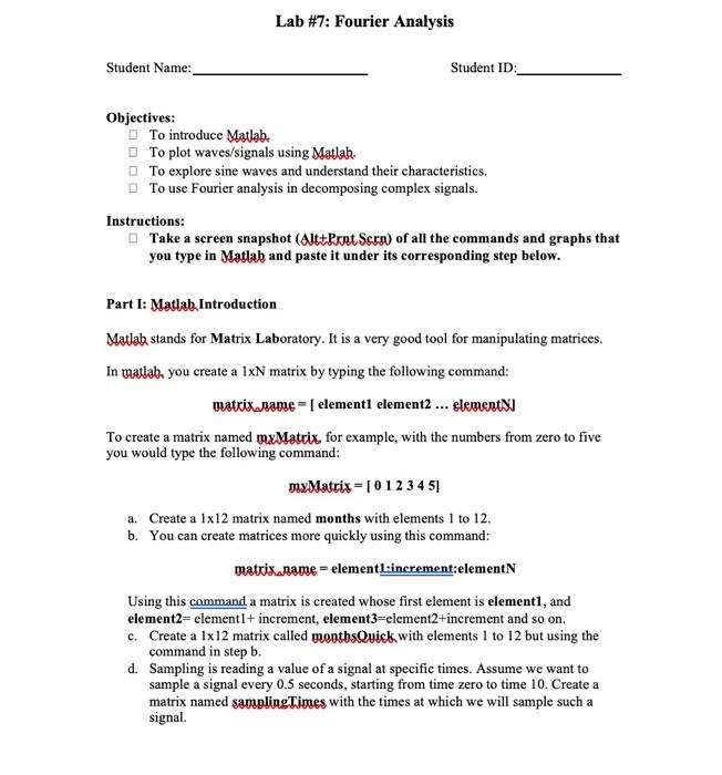
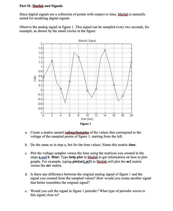
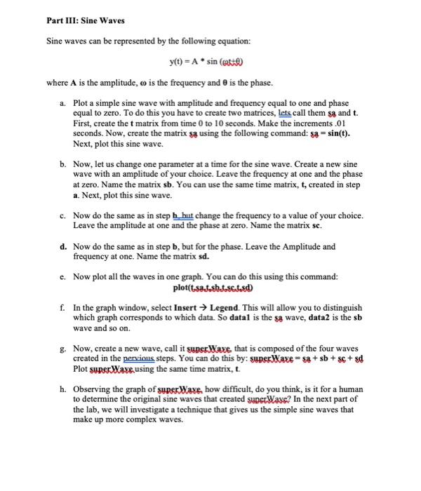
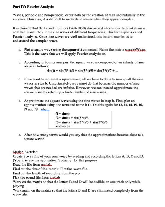
Lab #7: Fourier Analysis Student Name: Student ID: Objectives: To introduce Matlab To plot waves/signals using Matlab To explore sine waves and understand their characteristics. To use Fourier analysis in decomposing complex signals. Instructions: Take a screen snapshot (Alt+Pint Scra) of all the commands and graphs that you type in Matlab and paste it under its corresponding step below. Part I: Matlab Introduction Matlab stands for Matrix Laboratory. It is a very good tool for manipulating matrices. In matlab, you create a IxN matrix by typing the following command: matrix.name = ( elementi element2 ... elements To create a matrix named mx Matrix, for example, with the numbers from zero to five you would type the following command: my Matrix = [01 2 3 4 51 a. Create a 1x12 matrix named months with elements 1 to 12. b. You can create matrices more quickly using this command: matrix.name = elementL:increment:element Using this command a matrix is created whose first element is element1, and element2= elementl+ increment, element3-element2+increment and so on. c. Create a 1x 12 matrix called monthsQuick with elements 1 to 12 but using the command in step b. d. Sampling is reading a value of a signal at specific times. Assume we want to sample a signal every 0.5 seconds, starting from time zero to time 10. Create a matrix named sampling Times with the times at which we will sample such a signal. Part II: Matlab and Signals Since digital signals are a collection of points with respect to time, Mutab is naturally suited for modeling digital signals. Observe the analog signal in figure 1. This signal can be sampled every two seconds, for example, as shown by the small circles in the figure. Electric Signal 2 1.8 1.6 14 1.2 Volts 0.6 0.4 02 0 -02 -0.4 06 0 -1 0 4 6 14 16 18 20 8 10 12 time (sec) Figure 1 a. Create a matrix named voltage Samples of the values that correspond to the voltage of the sampled points of figure 1, starting from the left. b. Do the same as in step a, but for the time values. Name this matrix time. c. Plot the voltage samples versus the time using the matrices you created in the steps aand b. Hint: Type help plot in Matlab to get information on how to plot graphs. For example, typing plot(m1m2) in Matlab will plot the m2 matrix versus the ml matrix d. Is there any difference between the original analog signal of figure 1 and the signal you created from the sampled values? How would you create another signal that better resembles the original signal? e. Would you call the signal in figure I periodic? What type of periodic waves is this signal close to? Part III: Sine Waves Sine waves can be represented by the following equation: y(t) = A * sin (til) where A is the amplitude, is the frequency and is the phase. a. Plot a simple sine wave with amplitude and frequency equal to one and phase equal to zero. To do this you have to create two matrices, lets call them sa and t. First, create the t matrix from time 0 to 10 seconds. Make the increments.01 seconds. Now, create the matrix s using the following command: sa = sin(t). Next, plot this sine wave. b. Now, let us change one parameter at a time for the sine wave. Create a new sine wave with an amplitude of your choice. Leave the frequency at one and the phase at zero. Name the matrix sb. You can use the same time matrix, t, created in step a. Next, plot this sine wave. c. Now do the same as in step b_hut change the frequency to a value of your choice. Leave the amplitude at one and the phase at zero. Name the matrix se. d. Now do the same as in step b, but for the phase. Leave the Amplitude and frequency at one. Name the matrix sd. e. Now plot all the waves in one graph. You can do this using this command: plot(t.saj.sh.sc.Jesd) f. In the graph window, select Insert Legend. This will allow you to distinguish which graph corresponds to which data. So datal is the sa wave, data2 is the sb wave and so on. g. Now, create a new wave, call it super Waxe, that is composed of the four waves created in the perxious, steps. You can do this by: superWaxe = sa + sb + s + sd Plot superWave using the same time matrix, t. h. Observing the graph of superWave, how difficult, do you think, is it for a human to determine the original sine waves that created superWaxe? In the next part of the lab, we will investigate a technique that gives us the simple sine waves that make up more complex waves. Part IV: Fourier Analysis Waves, periodic and non-periodic, occur both by the creation of man and naturally in the universe. However, it is difficult to understand waves when they appear complex It is claimed that the French Fourier (1768-1830) discovered a technique to breakdown a complex wave into simple sine waves of different frequencies. This technique is called Fourier analysis. Since sine waves are well-understood, this in turn enables us to understand the complex wave. a. Plot a square wave using the square(t) command. Name the matrix square Wave. This is the wave that we will apply Fourier analysis on. b. According to Fourier analysis, the square wave is composed of an infinity of sine wave as follows: sin(t) + sin(3*t)/3 + sin(5*t)/5 + sin(7*t3/7 + .. c. If we want to represent a square wave, all we have to do is to sum up all the sine waves in step b. Unfortunately, we cannot do that because the number of sine waves that are needed are infinite. However, we can instead approximate the square wave by selecting a finite number of sine waves. d. Approximate the square wave using the sine waves in step b. First, plot an approximation using one term and name it fl. Do this again for 12, 13, 14, 15, 16, 17 and 18, where fl=sin(t) 12-sin(t) + sin(3*t)/3 13= sin(t) + sin(3*1)/3 + sin(5*t)/5 and so on. e. After how many terms would you say that the approximations became close to a square wave? Matab Exercise: Create a .wav file of your own voice by reading and recording the letters A, B, C and D. (You may use the application audacity for this purpose Read the file from matlab. Find out the size of the matrix. Plot the wave file. Find out the length of recording from the plot. Play the sound file from matlab Work on the matrix so that the letters B and D will be audible on one track only while playing Work again on the matrix so that the letters B and D are eliminated completely from the wave file. Turn in: 1. Complete all steps as listed in this lab document, provide screen shots and answer the questions. 2. Matlak code and screen shots for all of the activities listed in the exercise. 3. Reform Fourier analysis by creating a model in the simulink