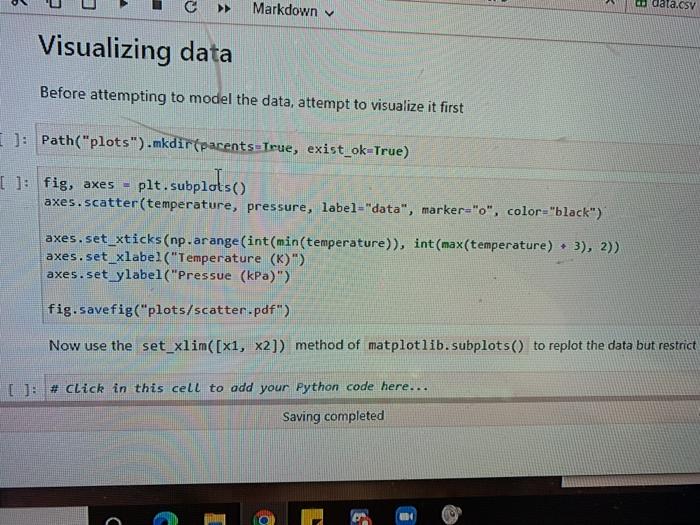
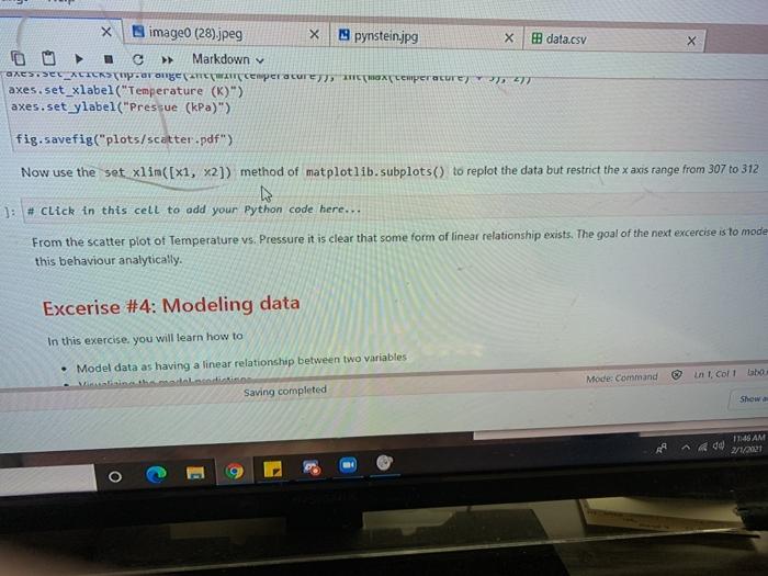
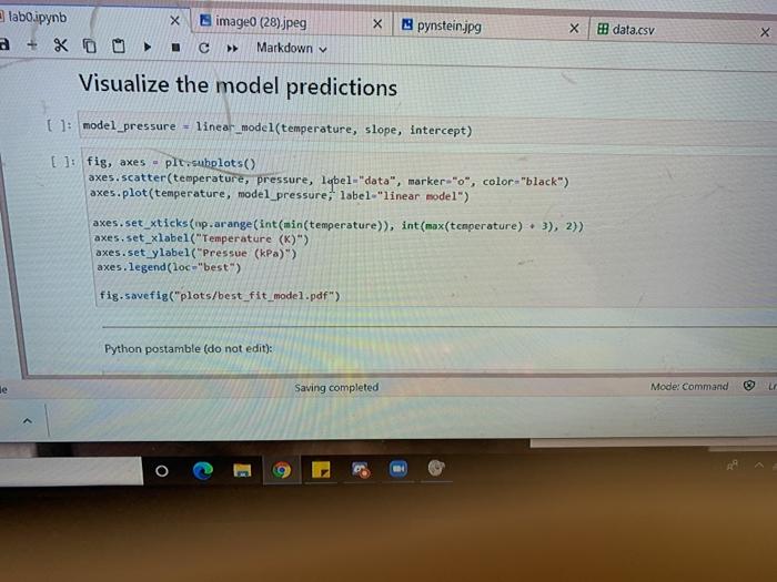
Markdown data.CSV Visualizing data Before attempting to model the data, attempt to visualize it first I]: Path("plots").mkdir(parents True, exist_ok=True) [ ]: fig, axes - plt.subplotso) axes. scatter(temperature, pressure, label="data", marker="o", color="black") +3), 2)) axes.set_xticks(np.arange(int(min(temperature)), int(max(temperature) axes.set_xlabel("Temperature (K)") axes.set_ylabel("Pressue (kPa)") fig.savefig("plots/scatter-pdf") Now use the set_xlim([x1, x2]) method of matplotlib.subplots() to replot the data but restrict [] # Click in this cell to add your Python code here... Saving completed C data.csv X image0 (28).jpeg X 9 pynstein.jpg Markdown axts._XCIT.avong Tenperace Hoxtemperature 27 axes.set_xlabel("Temperature (K)") axes.set ylabel("Pressue (kPa)") fig.savefig("plots/scatter.pdf") Now use the set xlim([x1, x2]) method of matplotlib.subplots() to replot the data but restrict the x axis range from 307 to 312 ]: # Click in this cell to add your Python code here... From the scatter plot of Temperature vs. Pressure it is clear that some form of linear relationship exists. The goal of the next excercise is to mode this behaviour analytically. Excerise #4: Modeling data In this exercise, you will learn how to Model data as having a linear relationship between two variables Mode Command in collabo Saving completed Showa do 11:48 AM 2/1/2021 E g labo apynb a + x image0 (28).jpeg C Markdown pynstein.jpg X data.csv X Visualize the model predictions U : model_pressure - linear_model(temperature, slope, intercept) []: fig, axes - pit, subplots() axes.scatter(temperature, pressure, lubel"data", marker="0", color="black") axes.plot(temperature, model pressure, label="linear model") axes.set_xticks(np.arange(int(min(temperature)), int(max(temperature). 3), 2)) axes.set_xlabel("Temperature (K)") axes.set ylabel("Pressue (kPa)") axes. legend (loc="best") fig.savefig("plots/best_fit_model.pdf) Python postamble (do not edit): Saving completed Mode: Command o Markdown data.CSV Visualizing data Before attempting to model the data, attempt to visualize it first I]: Path("plots").mkdir(parents True, exist_ok=True) [ ]: fig, axes - plt.subplotso) axes. scatter(temperature, pressure, label="data", marker="o", color="black") +3), 2)) axes.set_xticks(np.arange(int(min(temperature)), int(max(temperature) axes.set_xlabel("Temperature (K)") axes.set_ylabel("Pressue (kPa)") fig.savefig("plots/scatter-pdf") Now use the set_xlim([x1, x2]) method of matplotlib.subplots() to replot the data but restrict [] # Click in this cell to add your Python code here... Saving completed C data.csv X image0 (28).jpeg X 9 pynstein.jpg Markdown axts._XCIT.avong Tenperace Hoxtemperature 27 axes.set_xlabel("Temperature (K)") axes.set ylabel("Pressue (kPa)") fig.savefig("plots/scatter.pdf") Now use the set xlim([x1, x2]) method of matplotlib.subplots() to replot the data but restrict the x axis range from 307 to 312 ]: # Click in this cell to add your Python code here... From the scatter plot of Temperature vs. Pressure it is clear that some form of linear relationship exists. The goal of the next excercise is to mode this behaviour analytically. Excerise #4: Modeling data In this exercise, you will learn how to Model data as having a linear relationship between two variables Mode Command in collabo Saving completed Showa do 11:48 AM 2/1/2021 E g labo apynb a + x image0 (28).jpeg C Markdown pynstein.jpg X data.csv X Visualize the model predictions U : model_pressure - linear_model(temperature, slope, intercept) []: fig, axes - pit, subplots() axes.scatter(temperature, pressure, lubel"data", marker="0", color="black") axes.plot(temperature, model pressure, label="linear model") axes.set_xticks(np.arange(int(min(temperature)), int(max(temperature). 3), 2)) axes.set_xlabel("Temperature (K)") axes.set ylabel("Pressue (kPa)") axes. legend (loc="best") fig.savefig("plots/best_fit_model.pdf) Python postamble (do not edit): Saving completed Mode: Command o