MATLAB ASSIGN 1- Follow Directions and Complete. Will Thumbs Up!

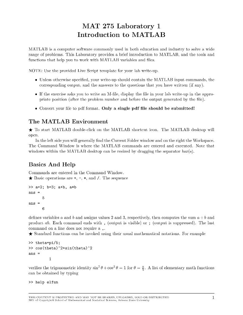
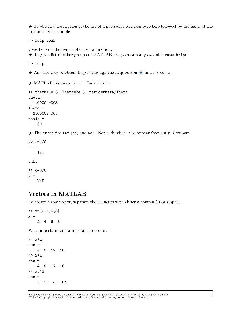
Directions: Unless otherwise specified, your write-up should contain the MATLAB input commands, the corresponding output, and the answers to the questions that you have written (if any). If the exercise asks you to write an M-file, display the file in your lab write-up in the appropriate position (after the problem number and before the output generated by the file). Convert your file to pdf format. Only a single pdf file should be submitted!

So Follow the Directions and copy the template as shown. Put your answers to the 6 exercises into the template that you made that looks exactly like the one given.

TEMPLATE TO COPY ON MATLAB

Directions For the 6 Exercises

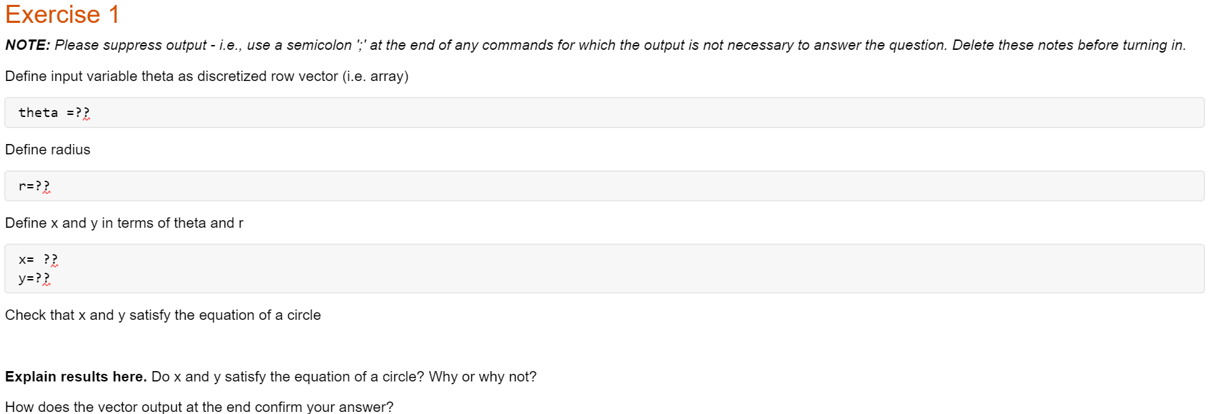
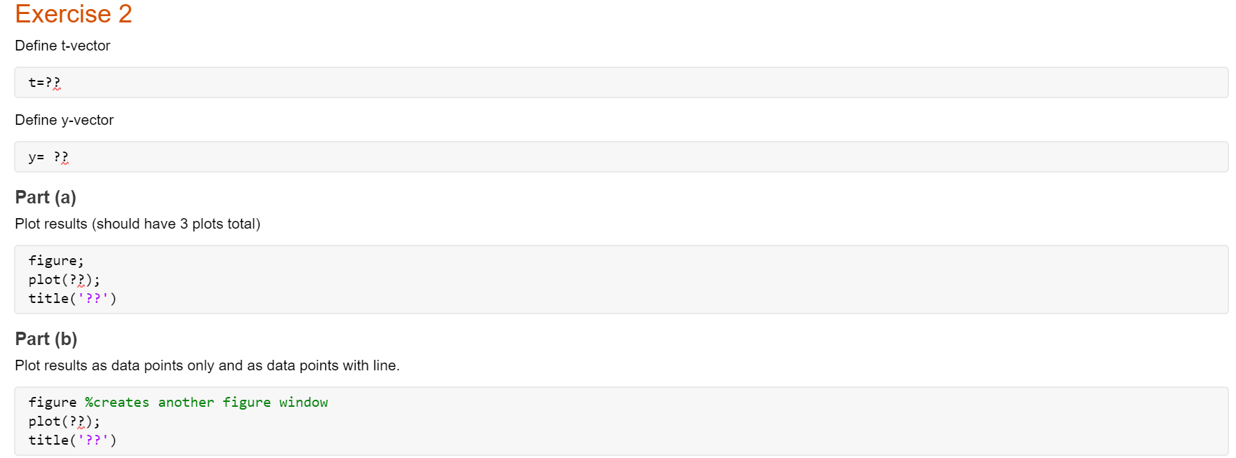
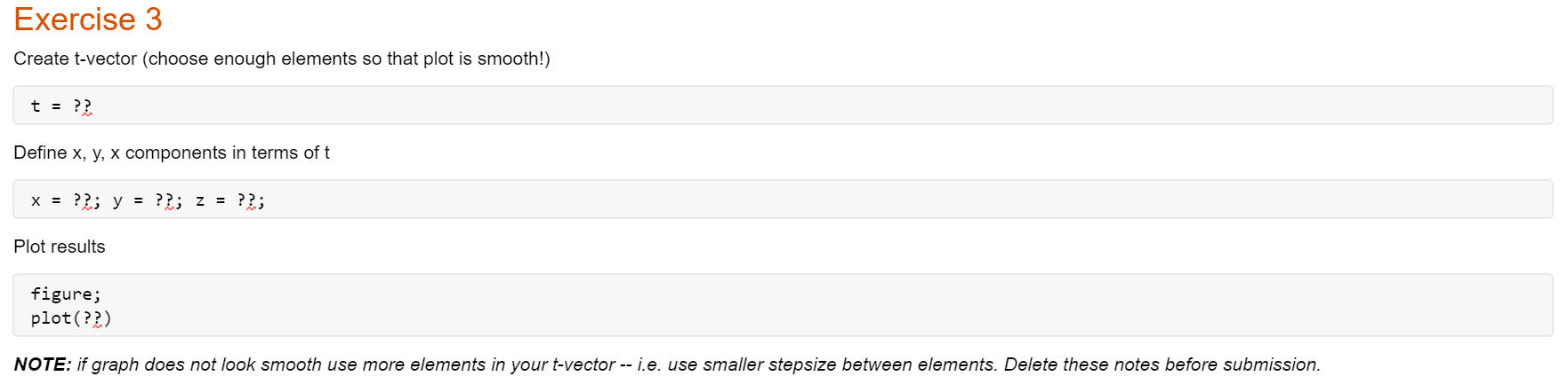
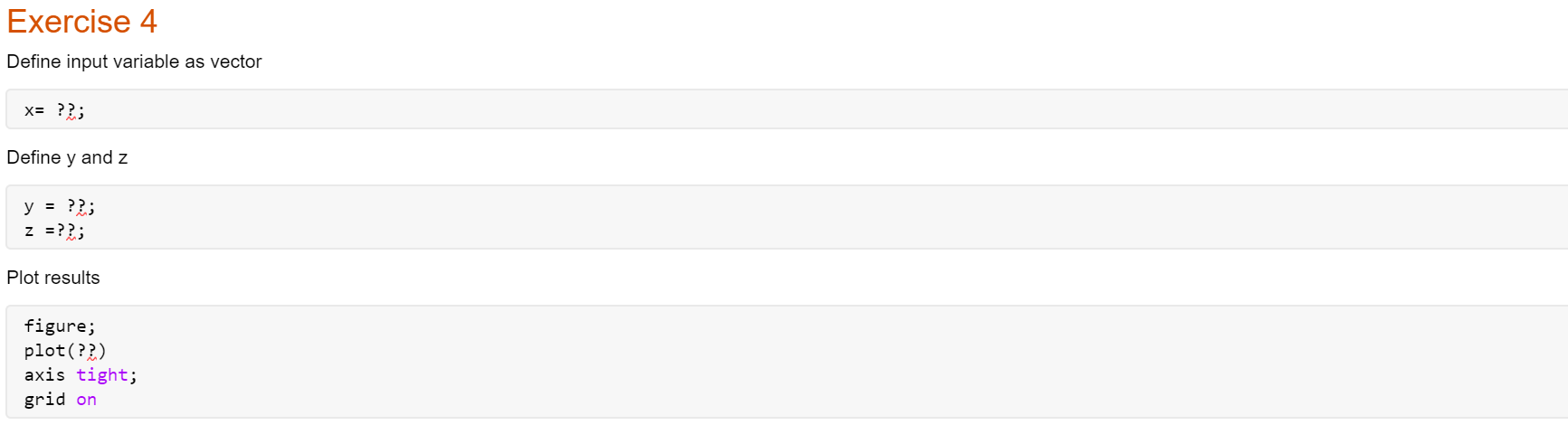
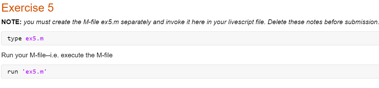
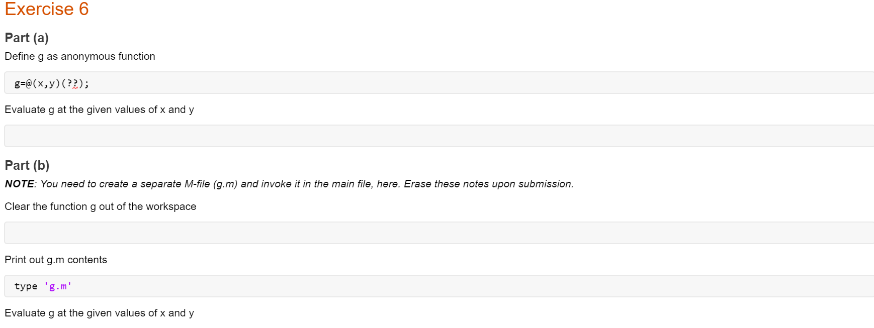
Exercise 1 NOTE: Please suppress output - i.e., use a semicolon ';' at the end of any commands for which the output is not necessary to answer the question. Delete these notes before turning in. Define input variable theta as discretized row vector (i.e. array) theta =?? Define radius r=?? Define x and y in terms of theta andr x= ?? y=?? Check that x and y satisfy the equation of a circle Explain results here. Do x and y satisfy the equation of a circle? Why or why not? How does the vector output at the end confirm your answer? Exercise 2 Define t-vector t=?? Define y-vector y= ?? Part (a) Plot results (should have 3 plots total) figure; plot(??); title('??') Part (b) Plot results as data points only and as data points with line. figure %creates another figure window plot(??); title('??') Exercise 3 Create t-vector (choose enough elements so that plot is smooth!) t = ?? Define x, y, x components in terms of t x = ??; y = ??; z = ??; Plot results figure; plot(??) NOTE: if graph does not look smooth use more elements in your t-vector -- i.e. use smaller stepsize between elements. Delete these notes before submission. Exercise 4 Define input variable as vector x= ??; Define y and z y = ??; z =??; Plot results figure; plot(??) axis tight; grid on Exercise 5 NOTE: you must create the M-file ex5.m separately and invoke it here in your livescript file. Delete these notes before submission. type ex5.m Run your M-file--i.e. execute the M-file run 'ex5.m' Exercise 6 Part (a) Define g as anonymous function g=@(x,y) (??); Evaluate g at the given values of x and y Part (b) NOTE: You need to create a separate M-file (g.m) and invoke it in the main file, here. Erase these notes upon submission. Clear the function g out of the workspace Print out g.m contents type 'g.m' Evaluate g at the given values of x and y MAT 275 Laboratory 1 Introduction to MATLAB MATLAB is a computer software commonly used in both education and industry to solve a wide range of problems. This Laboratory provides a brief introduction to MATLAB, and the tools and functions that help you to work with MATLAB variables and files. NOTE: Use the provided Live Script template for your lab write-up. Unless otherwise specificd, your write-up should contain the MATLAB input commands, the corresponding output, and the answers to the questions that you have written (if any). If the exercise asks you to write an M-file, clisplay the file in your lah write-up in the appro- priate position (after the problem number and before the output generated by the file). Convert your file to pdf format. Only a single pdf file should be submitted! The MATLAB Environment * To start MATLAB double-click on the MATLAB shortcut icon. The MATLAB desktop will open In the left side you will generally find the Current Folder window and on the right the Workspace. The Command Window is where the MATLAB commands are cntcrcd and cxccuted. Note that windows within the MATLAB desktop can be resized by dragging the separator bar(s). Basics And Help Commands are entered in the Command Window * Basic operations are +, -- *, und /. The sequence >>> a=2; b=3; a+b, a*b ans = 5 ans = 6 defines variables a and b and assigns values 2 and 3, respectively, then computes the sum a +b and prodlucu ah. Each command euds will , (output is visible) or ; (output is suppressed). The last command on a line does not require a .. * Standard functions can be invoked using their usual mathematical notations. For example >> theta=pi/5; >> cos (theta) 2+sin(theta) 2 ans = 1 verifies the trigonometric identity sin 0 + cos20 = 1 for 0 = A list of elementary math functions can be obtained by typing >> help elfun THIS CONTENT IS PROTECTED AND MAY NOT BE SHARED, UPLOADEN, SOLD OR DISTRIBUTED 2021 v2 Copyright Scheel of Vistatical and Statistical Scienos, Arizona State University * To obtain a description of the use of a particular function type help followed by the name of the function. For example >> help cosh gives help on the hyperbolic cosine function. To get a list of other groups of MATLAB programs already available enter help: >> help * Another way to obtain help is through the help button in the toolbar. * MATLAB is case-sensitive. For example >> theta=1e-3, Theta=2e-5, ratio=theta/Theta theta = 1.0000e-003 Theta = 2.00000-005 ratio = 50 * The quantities Inf (0) and NaN (Not a Number) also appear frequently. Compare >> c=1/0 C = Inf with >> d=0/0 d = NaN Vectors in MATLAB To create a row vector, separate the elements with either a comma (,) or a space >> x=[2,4,6,8) 2 4 6 8 We can perform operations on the vector: 12 16 >> X+X ans = 4 8 >> 2*x ans = 4 8 >> X-2 12 16 ans = 4 16 36 64 THIS CONTENT IS PROTECTED AND MAY NOT BE SHARED, UPLOADEN, SOLD OR DISTRIBUTED 2021 v2 Copyrigh School of Mathematical and Statistical Sciences, Arizona State University 2 Each entry of the vector x is squared. ans = 4 16 36 64 Each entry of the vector x is multiplied by itself. Note that in the above example multiplication (*) and exponentitation are proceeded by a dot (.) in order for the expression to be evaluated for each component (entry) of r. This is necessary to prevent MATLAB from interpreting these symbols as standard linear algebra symbols operating on arrays. Because the slaudard + anul - operations ou arrays already work componentwise, a dol is not necessary for + and - We can apply MATLAB built in functions to the vector >> sqrt(x) ans = 1.4142 2.0000 2.4495 2.8284 Exercise 1 All points with coordinates 2. - r cos(0) and y - rsin(), where r is a constant, lie on a circle with radius r. i.e. satisfy the equation z2 + y2 = 72 Create a row vector for 8 with the values 8 -0,56 and Take r - 7 and compute the row vectors x audy. Now check that I and y indeed satisfy the equation of a circle by computing the radius r=V2 + y Hint: To calculate r you will need the array operator for squaring r and y. Of course, you could also compute z by x.*x. The colon (:) operator and the linspace command Rather than manually entering cach entry of a vector, we can create equidistant vectors by using the colon : operator: >> X = 0:2:2 0 0.2000 0.4000 0.6000 0.8000 1.0000 1.2000 1.4000 1.6000 1.8000 2.0000 MATLAB creates a vector with the first entry equal to 0. the last entry equal to 2 and with equidistant entries by increments of 0.2. The most general form of the command is : : where is the first entry to be put in the vector, the next entry will be + (step), the next entry + 2 and so on. The last entry in the vector is the largest value of + P less than or equal to : : ) For example >> x=linspace(0,2,11) generates the same output vector x. THIS CONTENT IS PROTECTED AND MAY NOT BE SHARED, UPLOADEN, SOLD OR DISTRIBUTED 2021 v2 Copyright Scheel of Vistatical and Statistical Scienos, Arizona State University 3 Plotting with MATLAB * To plot a function you have to crcate two arrays (vectors): onc containing the abscissac, the other the corresponding function values. Both arrays should have the same length. For example, consider plotting the function 2.- sin() + " y = f(2)= -1 for 0> x= 0:0.1:2 0.2000 0.3000 0.4000 0.5000 0.6000 Columns 1 through 7 0 0.1000 Columns 8 through 14 0.7000 0.8000 Columns 15 through 21 1.4000 1.5000 0.9000 1.0000 1.1000 1.2000 1.3000 1.6000 1.7000 1.8000 1.9000 2.0000 * The output for x can be suppressed (by adding ; at the end of the command). Alternatively, we can also display the output in a more compact form by entering >> format compact This format suppresses unnecessary lines and allows more information to show on the screen. * To evaluate the function f simultaneously at all the values contained in 1, type >> y=(x. 2-sin (pi. **) +exp(x))/(x-1) y = Columns 1 through 6 -1.0000 -0.8957 -0.8420 -0.9012 -1.1679 -1.7974 Columns 7 through 12 -3.0777 -5.6491 -11.3888 -29.6059 Inf 45.2318 Columns 13 through 18 26.7395 20.5610 17.4156 15.4634 14.1068 13.1042 Columns 19 through 21 12.3468 11.7832 11.3891 Note that the function becomes infinite at :r = 1 (vertical asymptote). The array y inherits the dimension of c, namely 1 (row) by 21 (columns). Note also the use of parentheses. IMPORTANT REMARK In the above example *. / and are preceded by a dot. in order for the expression to be evaluated for cach component (entry) of r. The command >> plot(x,y) creates a Figure window and shows the function (see Fig. 1). Note how the curve is not smooth. The reason is that the vector x does not have enough entries. We can see more clearly how MATLAB plots the curve, by plotting circles 'o' at each of the ordered pairs (w.y) and connecting the circles (see Fig. 2): >> plot(x,y,'-') THIS CONTENT IS PROTECTED AND MAY NOT BE SHARED, UPLOADED, SOLD OR DISTRIBUTED 2021 v2 Copyright Scheel of Vistatical and Statistical Scienos, Arizona State University 1 Figure 1 Figure 2 The figure can be edited and manipulated using the Figure window memus and buttons. Alternately, properties of the figure can also be defined directly at the command line: >> x=0:.01:2; % create a vector X with more entries >> y=(x.2-sin(pi.*x) + exp(x))./(x-1); %recompute y >> plot(x,y,'r-', 'LineWidth',2); %plot in red with a thicker line >> axis ([0,2,-10,20]); % change the window to [0,2] x [-10,20] >> grid on; % add a grid >> title('f(x)=(x 2-sin(\pi x) + x)/(x-1)'); % create a >> xlabel('x'); ylabel('y'); % create labels title T TEO.I devu... NODE Figure 3 Remarks: The number of r-values has been increased for a smoother curve (riote that the stepsize is now .01 rather than .1). The vector y is recomputed using the new vector . The option 'I-' plots the curve in red. 'LineWidth:2 sets the width of the line to 2 points (the default is 0.5). The range of 2 and y values has been reset using axis((0,2,-10,20]) (always a good idea in the presence of vertical asymptotes). The general command is axis ([xmin, xmax, yain, ymax]). THIS CONTENT IS PROTECTED AND MAY NOT BE SHARED, UPLOADEN, SOLD OR DISTRIBUTED 2021 v2 Copyright Scheel of Vistatical and Statistical Scienos, Arizona State University 5 The command grid on adds a grid to the plot. . A title and labels have been added. The resulting new plot is shown in Fig. 3. For more options type help plot in the Command Windos. Exercise 2 Use the linspace command of the colon operator to create a vector t with entries 4/10 cos(2+ 2, 2.1, 2.2...., 10, and define the function y= (make sure you ise ";" lo suppress the 0.873 +11 output for both t and y). (a) Plot the function y in black and include a title with the expression for y). (b) Make the same plot as in part (a), but rather than displaying the graph as a curve, show the urconnected data points. To display the data points with small circles, use plot(t,y,'o'). Now combine the two plots with the command plot(t,y,'o-) to show the line through the data points as well as the distinct data points. The plot3 command Space curves can be easily plotted in MATLAB using the plot3 command. For instance, suppose we want to plot the space curve defined by the parametric equations = sin(32) cos(/), y =sin(36) sin(). z = cos in the interval 0 > t = 0:0.01:2*pi; >> x=sin(3*t).*cos(t); >> y=sin(3*t).*sin(t); >> z=cos (t); We then use the plot3 command to plot the space curve: >> plot3(x,y,z); >> grid on; Figure 1 The command grid on adds a grid to the plot. The resulting plot is shown in Fig. 4. Exercise 3 Use the command plot3(x,y,z) to plot the circular helix x = 3 cos(7t), y = 3 sin(7t), 2 = 2t, O55. Add a grid to the plot using the command grid on. NOTE: Use semicolon to suppress the outpuu, when you define the vectors I, II, yan . Make sure you use enough points for your graph so that the resulting curve is nice and smooth. THIS CONTENT IS PROTECTED AND MAY NOT BE SHARED, LIOADED, SOLD OR DISTRIBUTED 2021 v2 Copyright Scheel of Vistatical and Statistical Scienos, Arizona State University 6 Combining multiple plots By default new plots clear exisl.ing plots and reset axes properties, such as the title. Ilowever there are different ways to combine multiple plots in the same axes. The hold on command Suppose we want to plot the functious y = cos(x) and y = cos(2:) in the interval -, > x=2; y=myfunction(x) y = 11.3891 A script can be called from another script or function in which case it is local to that function). Il' any modification is made, the script or function can be re-executed by simply relyping the script or function name in the Command Window or use the up-arrow on the keyboard to browse through past commands). IMPORTANT REMARK By default MATLAB saves files in the Current Polder. To change directory use the Current Directory box on top of the MATLAB desktop. 9 THIS CONTENT IS PROTECTED AND MAY NOT BE SHARED, UPLOADEN, SOLD OR DISTRIBUTED 2021 v2 Copyright Scheel of Vistatical and Statistical Scienos, Arizona State University Exercise 5 dy The general solution to the differential equation = -0.2 - 13.7" + 4 cos(T) is dar y() - - - 13 x 2 + 4 sin(x) +C with yo) C. The goal of this exercise is to write a script file to plot the solutions to the differential equation in the interval 0 > f (2,1) % evaluate the function f at t = 2 and y = 1 ans 3 10 THIS CONTENT IS PROTECTED AND MAY NOT BE SHARED, UPLOADEN, SOLD OR DISTRIBUTED 2021 v2 Copyright Scheel of Vistatical and Statistical Scienos, Arizona State University or we can define the function directly on the command line as an anonymous function. An anony- mous function is a function that is not stored in a program file, but is associatel with a variable whose data type is function handle. Anonymous functions can accept inputs and return outputs, just as standard functions do. Ilowever, they can contain only a single executable statement. For example: >> f = @(t,y) (t-2-y) % define f(t,y)=="2-y as anonymous function The parentheses () immediately after the operator include the function input arguments. This anonymous function accepts two inputs t and y and implicitly returns a single output, the value of % evaluate the function f at t = 2 and y = 1 > > f (2,1) ans = 3 * CAUTION! The names of script or function M-files must begin with a letter. The rest of the characters may include digits and the underscore character. You may not use periods in the name other than the last one in 'mand the name cannot contain blank spaces. Avoid name clashes with built-in functions. It is a good idea to first check i a function or a script file of the proposed nane already exists. You can do this with the command exist('name'), which relurux zero i nothing with name name exists. NEVER nome a script file or function file the same as the name of the variable it computes. When MATLAB looks for a name, it first searches the list of variables in the workspacc. If a variable of the same name as the script file exists. MATLAB will never be able to access the script file. Exercise 6 ? cos(Gare?) (a) Enter the function g(x,y) = +7 as an anonymous function. Evaluate the function at 1 - 2 and y=-5 by entering g(2, -5) in the command window. (b) Type clear g to clear the value of the function from part (a). Now write a function M file 22 cos(62c2v) for the function glar,y) = Save the file is g.n (include the M-file in your y 25+7 report). Evaluate the function al. 1 = 2 and y= -5 by entering g(2,-5) in the command window. + 11 THIS CONTENT IS PROTECTED AND MAY NOT BE SHARED, UPLOADED, SOLD OR DISTRIBUTED 2021 v2 Copyright Scheel of Vistatical and Statistical Scienos, Arizona State University Exercise 1 NOTE: Please suppress output - i.e., use a semicolon ';' at the end of any commands for which the output is not necessary to answer the question. Delete these notes before turning in. Define input variable theta as discretized row vector (i.e. array) theta =?? Define radius r=?? Define x and y in terms of theta andr x= ?? y=?? Check that x and y satisfy the equation of a circle Explain results here. Do x and y satisfy the equation of a circle? Why or why not? How does the vector output at the end confirm your answer? Exercise 2 Define t-vector t=?? Define y-vector y= ?? Part (a) Plot results (should have 3 plots total) figure; plot(??); title('??') Part (b) Plot results as data points only and as data points with line. figure %creates another figure window plot(??); title('??') Exercise 3 Create t-vector (choose enough elements so that plot is smooth!) t = ?? Define x, y, x components in terms of t x = ??; y = ??; z = ??; Plot results figure; plot(??) NOTE: if graph does not look smooth use more elements in your t-vector -- i.e. use smaller stepsize between elements. Delete these notes before submission. Exercise 4 Define input variable as vector x= ??; Define y and z y = ??; z =??; Plot results figure; plot(??) axis tight; grid on Exercise 5 NOTE: you must create the M-file ex5.m separately and invoke it here in your livescript file. Delete these notes before submission. type ex5.m Run your M-file--i.e. execute the M-file run 'ex5.m' Exercise 6 Part (a) Define g as anonymous function g=@(x,y) (??); Evaluate g at the given values of x and y Part (b) NOTE: You need to create a separate M-file (g.m) and invoke it in the main file, here. Erase these notes upon submission. Clear the function g out of the workspace Print out g.m contents type 'g.m' Evaluate g at the given values of x and y MAT 275 Laboratory 1 Introduction to MATLAB MATLAB is a computer software commonly used in both education and industry to solve a wide range of problems. This Laboratory provides a brief introduction to MATLAB, and the tools and functions that help you to work with MATLAB variables and files. NOTE: Use the provided Live Script template for your lab write-up. Unless otherwise specificd, your write-up should contain the MATLAB input commands, the corresponding output, and the answers to the questions that you have written (if any). If the exercise asks you to write an M-file, clisplay the file in your lah write-up in the appro- priate position (after the problem number and before the output generated by the file). Convert your file to pdf format. Only a single pdf file should be submitted! The MATLAB Environment * To start MATLAB double-click on the MATLAB shortcut icon. The MATLAB desktop will open In the left side you will generally find the Current Folder window and on the right the Workspace. The Command Window is where the MATLAB commands are cntcrcd and cxccuted. Note that windows within the MATLAB desktop can be resized by dragging the separator bar(s). Basics And Help Commands are entered in the Command Window * Basic operations are +, -- *, und /. The sequence >>> a=2; b=3; a+b, a*b ans = 5 ans = 6 defines variables a and b and assigns values 2 and 3, respectively, then computes the sum a +b and prodlucu ah. Each command euds will , (output is visible) or ; (output is suppressed). The last command on a line does not require a .. * Standard functions can be invoked using their usual mathematical notations. For example >> theta=pi/5; >> cos (theta) 2+sin(theta) 2 ans = 1 verifies the trigonometric identity sin 0 + cos20 = 1 for 0 = A list of elementary math functions can be obtained by typing >> help elfun THIS CONTENT IS PROTECTED AND MAY NOT BE SHARED, UPLOADEN, SOLD OR DISTRIBUTED 2021 v2 Copyright Scheel of Vistatical and Statistical Scienos, Arizona State University * To obtain a description of the use of a particular function type help followed by the name of the function. For example >> help cosh gives help on the hyperbolic cosine function. To get a list of other groups of MATLAB programs already available enter help: >> help * Another way to obtain help is through the help button in the toolbar. * MATLAB is case-sensitive. For example >> theta=1e-3, Theta=2e-5, ratio=theta/Theta theta = 1.0000e-003 Theta = 2.00000-005 ratio = 50 * The quantities Inf (0) and NaN (Not a Number) also appear frequently. Compare >> c=1/0 C = Inf with >> d=0/0 d = NaN Vectors in MATLAB To create a row vector, separate the elements with either a comma (,) or a space >> x=[2,4,6,8) 2 4 6 8 We can perform operations on the vector: 12 16 >> X+X ans = 4 8 >> 2*x ans = 4 8 >> X-2 12 16 ans = 4 16 36 64 THIS CONTENT IS PROTECTED AND MAY NOT BE SHARED, UPLOADEN, SOLD OR DISTRIBUTED 2021 v2 Copyrigh School of Mathematical and Statistical Sciences, Arizona State University 2 Each entry of the vector x is squared. ans = 4 16 36 64 Each entry of the vector x is multiplied by itself. Note that in the above example multiplication (*) and exponentitation are proceeded by a dot (.) in order for the expression to be evaluated for each component (entry) of r. This is necessary to prevent MATLAB from interpreting these symbols as standard linear algebra symbols operating on arrays. Because the slaudard + anul - operations ou arrays already work componentwise, a dol is not necessary for + and - We can apply MATLAB built in functions to the vector >> sqrt(x) ans = 1.4142 2.0000 2.4495 2.8284 Exercise 1 All points with coordinates 2. - r cos(0) and y - rsin(), where r is a constant, lie on a circle with radius r. i.e. satisfy the equation z2 + y2 = 72 Create a row vector for 8 with the values 8 -0,56 and Take r - 7 and compute the row vectors x audy. Now check that I and y indeed satisfy the equation of a circle by computing the radius r=V2 + y Hint: To calculate r you will need the array operator for squaring r and y. Of course, you could also compute z by x.*x. The colon (:) operator and the linspace command Rather than manually entering cach entry of a vector, we can create equidistant vectors by using the colon : operator: >> X = 0:2:2 0 0.2000 0.4000 0.6000 0.8000 1.0000 1.2000 1.4000 1.6000 1.8000 2.0000 MATLAB creates a vector with the first entry equal to 0. the last entry equal to 2 and with equidistant entries by increments of 0.2. The most general form of the command is : : where is the first entry to be put in the vector, the next entry will be + (step), the next entry + 2 and so on. The last entry in the vector is the largest value of + P less than or equal to : : ) For example >> x=linspace(0,2,11) generates the same output vector x. THIS CONTENT IS PROTECTED AND MAY NOT BE SHARED, UPLOADEN, SOLD OR DISTRIBUTED 2021 v2 Copyright Scheel of Vistatical and Statistical Scienos, Arizona State University 3 Plotting with MATLAB * To plot a function you have to crcate two arrays (vectors): onc containing the abscissac, the other the corresponding function values. Both arrays should have the same length. For example, consider plotting the function 2.- sin() + " y = f(2)= -1 for 0> x= 0:0.1:2 0.2000 0.3000 0.4000 0.5000 0.6000 Columns 1 through 7 0 0.1000 Columns 8 through 14 0.7000 0.8000 Columns 15 through 21 1.4000 1.5000 0.9000 1.0000 1.1000 1.2000 1.3000 1.6000 1.7000 1.8000 1.9000 2.0000 * The output for x can be suppressed (by adding ; at the end of the command). Alternatively, we can also display the output in a more compact form by entering >> format compact This format suppresses unnecessary lines and allows more information to show on the screen. * To evaluate the function f simultaneously at all the values contained in 1, type >> y=(x. 2-sin (pi. **) +exp(x))/(x-1) y = Columns 1 through 6 -1.0000 -0.8957 -0.8420 -0.9012 -1.1679 -1.7974 Columns 7 through 12 -3.0777 -5.6491 -11.3888 -29.6059 Inf 45.2318 Columns 13 through 18 26.7395 20.5610 17.4156 15.4634 14.1068 13.1042 Columns 19 through 21 12.3468 11.7832 11.3891 Note that the function becomes infinite at :r = 1 (vertical asymptote). The array y inherits the dimension of c, namely 1 (row) by 21 (columns). Note also the use of parentheses. IMPORTANT REMARK In the above example *. / and are preceded by a dot. in order for the expression to be evaluated for cach component (entry) of r. The command >> plot(x,y) creates a Figure window and shows the function (see Fig. 1). Note how the curve is not smooth. The reason is that the vector x does not have enough entries. We can see more clearly how MATLAB plots the curve, by plotting circles 'o' at each of the ordered pairs (w.y) and connecting the circles (see Fig. 2): >> plot(x,y,'-') THIS CONTENT IS PROTECTED AND MAY NOT BE SHARED, UPLOADED, SOLD OR DISTRIBUTED 2021 v2 Copyright Scheel of Vistatical and Statistical Scienos, Arizona State University 1 Figure 1 Figure 2 The figure can be edited and manipulated using the Figure window memus and buttons. Alternately, properties of the figure can also be defined directly at the command line: >> x=0:.01:2; % create a vector X with more entries >> y=(x.2-sin(pi.*x) + exp(x))./(x-1); %recompute y >> plot(x,y,'r-', 'LineWidth',2); %plot in red with a thicker line >> axis ([0,2,-10,20]); % change the window to [0,2] x [-10,20] >> grid on; % add a grid >> title('f(x)=(x 2-sin(\pi x) + x)/(x-1)'); % create a >> xlabel('x'); ylabel('y'); % create labels title T TEO.I devu... NODE Figure 3 Remarks: The number of r-values has been increased for a smoother curve (riote that the stepsize is now .01 rather than .1). The vector y is recomputed using the new vector . The option 'I-' plots the curve in red. 'LineWidth:2 sets the width of the line to 2 points (the default is 0.5). The range of 2 and y values has been reset using axis((0,2,-10,20]) (always a good idea in the presence of vertical asymptotes). The general command is axis ([xmin, xmax, yain, ymax]). THIS CONTENT IS PROTECTED AND MAY NOT BE SHARED, UPLOADEN, SOLD OR DISTRIBUTED 2021 v2 Copyright Scheel of Vistatical and Statistical Scienos, Arizona State University 5 The command grid on adds a grid to the plot. . A title and labels have been added. The resulting new plot is shown in Fig. 3. For more options type help plot in the Command Windos. Exercise 2 Use the linspace command of the colon operator to create a vector t with entries 4/10 cos(2+ 2, 2.1, 2.2...., 10, and define the function y= (make sure you ise ";" lo suppress the 0.873 +11 output for both t and y). (a) Plot the function y in black and include a title with the expression for y). (b) Make the same plot as in part (a), but rather than displaying the graph as a curve, show the urconnected data points. To display the data points with small circles, use plot(t,y,'o'). Now combine the two plots with the command plot(t,y,'o-) to show the line through the data points as well as the distinct data points. The plot3 command Space curves can be easily plotted in MATLAB using the plot3 command. For instance, suppose we want to plot the space curve defined by the parametric equations = sin(32) cos(/), y =sin(36) sin(). z = cos in the interval 0 > t = 0:0.01:2*pi; >> x=sin(3*t).*cos(t); >> y=sin(3*t).*sin(t); >> z=cos (t); We then use the plot3 command to plot the space curve: >> plot3(x,y,z); >> grid on; Figure 1 The command grid on adds a grid to the plot. The resulting plot is shown in Fig. 4. Exercise 3 Use the command plot3(x,y,z) to plot the circular helix x = 3 cos(7t), y = 3 sin(7t), 2 = 2t, O55. Add a grid to the plot using the command grid on. NOTE: Use semicolon to suppress the outpuu, when you define the vectors I, II, yan . Make sure you use enough points for your graph so that the resulting curve is nice and smooth. THIS CONTENT IS PROTECTED AND MAY NOT BE SHARED, LIOADED, SOLD OR DISTRIBUTED 2021 v2 Copyright Scheel of Vistatical and Statistical Scienos, Arizona State University 6 Combining multiple plots By default new plots clear exisl.ing plots and reset axes properties, such as the title. Ilowever there are different ways to combine multiple plots in the same axes. The hold on command Suppose we want to plot the functious y = cos(x) and y = cos(2:) in the interval -, > x=2; y=myfunction(x) y = 11.3891 A script can be called from another script or function in which case it is local to that function). Il' any modification is made, the script or function can be re-executed by simply relyping the script or function name in the Command Window or use the up-arrow on the keyboard to browse through past commands). IMPORTANT REMARK By default MATLAB saves files in the Current Polder. To change directory use the Current Directory box on top of the MATLAB desktop. 9 THIS CONTENT IS PROTECTED AND MAY NOT BE SHARED, UPLOADEN, SOLD OR DISTRIBUTED 2021 v2 Copyright Scheel of Vistatical and Statistical Scienos, Arizona State University Exercise 5 dy The general solution to the differential equation = -0.2 - 13.7" + 4 cos(T) is dar y() - - - 13 x 2 + 4 sin(x) +C with yo) C. The goal of this exercise is to write a script file to plot the solutions to the differential equation in the interval 0 > f (2,1) % evaluate the function f at t = 2 and y = 1 ans 3 10 THIS CONTENT IS PROTECTED AND MAY NOT BE SHARED, UPLOADEN, SOLD OR DISTRIBUTED 2021 v2 Copyright Scheel of Vistatical and Statistical Scienos, Arizona State University or we can define the function directly on the command line as an anonymous function. An anony- mous function is a function that is not stored in a program file, but is associatel with a variable whose data type is function handle. Anonymous functions can accept inputs and return outputs, just as standard functions do. Ilowever, they can contain only a single executable statement. For example: >> f = @(t,y) (t-2-y) % define f(t,y)=="2-y as anonymous function The parentheses () immediately after the operator include the function input arguments. This anonymous function accepts two inputs t and y and implicitly returns a single output, the value of % evaluate the function f at t = 2 and y = 1 > > f (2,1) ans = 3 * CAUTION! The names of script or function M-files must begin with a letter. The rest of the characters may include digits and the underscore character. You may not use periods in the name other than the last one in 'mand the name cannot contain blank spaces. Avoid name clashes with built-in functions. It is a good idea to first check i a function or a script file of the proposed nane already exists. You can do this with the command exist('name'), which relurux zero i nothing with name name exists. NEVER nome a script file or function file the same as the name of the variable it computes. When MATLAB looks for a name, it first searches the list of variables in the workspacc. If a variable of the same name as the script file exists. MATLAB will never be able to access the script file. Exercise 6 ? cos(Gare?) (a) Enter the function g(x,y) = +7 as an anonymous function. Evaluate the function at 1 - 2 and y=-5 by entering g(2, -5) in the command window. (b) Type clear g to clear the value of the function from part (a). Now write a function M file 22 cos(62c2v) for the function glar,y) = Save the file is g.n (include the M-file in your y 25+7 report). Evaluate the function al. 1 = 2 and y= -5 by entering g(2,-5) in the command window. + 11 THIS CONTENT IS PROTECTED AND MAY NOT BE SHARED, UPLOADED, SOLD OR DISTRIBUTED 2021 v2 Copyright Scheel of Vistatical and Statistical Scienos, Arizona State University