Matlab online
Questions


You are given the code below.


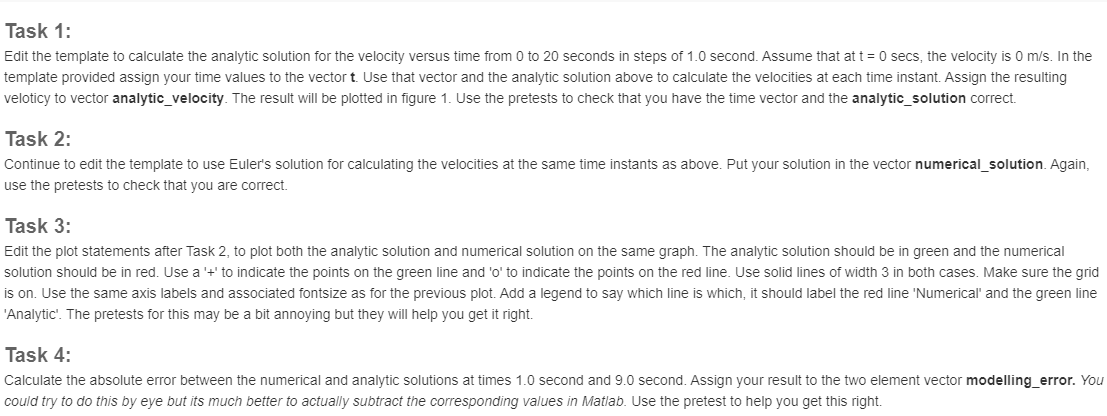
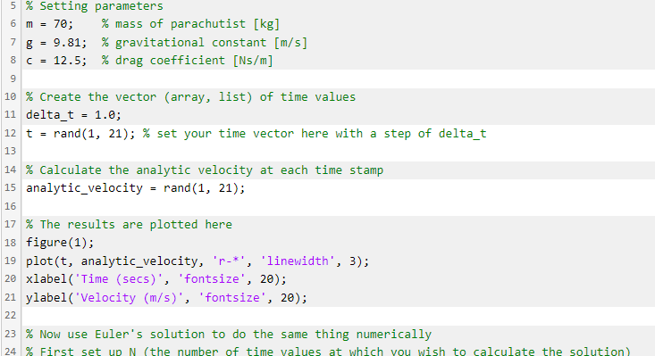
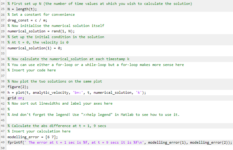
In the lectures, the governing ordinary differential equation (ODE) for the falling parachutist under idealised conditions was derived. It is repeated below for convenience: dv(t) cvt =g- dt m (1) The analytic solution was also derived as follows: vt) = mg 3 [1-6] (2) Where g is the gravitational constant (9.81 ms), m is the mass of parachutist (70 kg) and c is the drag coefficient (12.5 Ns/m). Task 1: Edit the template to calculate the analytic solution for the velocity versus time from 0 to 20 seconds in steps of 1.0 second. Assume that at t = 0 secs, the velocity is 0 m/s. In the template provided assign your time values to the vector t Use that vector and the analytic solution above to calculate the velocities at each time instant. Assign the resulting veloticy to vector analytic_velocity. The result will be plotted in figure 1. Use the pretests to check that you have the time vector and the analytic_solution correct. Task 2: Continue to edit the template to use Euler's solution for calculating the velocities at the same time instants as above. Put your solution in the vector numerical_solution. Again, use the pretests to check that you are correct. Task 3: Edit the plot statements after Task 2, to plot both the analytic solution and numerical solution on the same graph. The analytic solution should be in green and the numerical solution should be in red. Use a '+' to indicate the points on the green line and 'o' to indicate the points on the red line. Use solid lines of width 3 in both cases. Make sure the grid is on. Use the same axis labels and associated fontsize as for the previous plot. Add a legend to say which line is which, it should label the red line 'Numerical and the green line 'Analytic'. The pretests for this may be a bit annoying but they will help you get it right. Task 4: Calculate the absolute error between the numerical and analytic solutions at times 1.0 second and 9.0 second. Assign your result to the two element vector modelling_error. You could try to do this by eye but its much better to actually subtract the corresponding values in Matlab. Use the pretest to help you get this right. 6 ms 5 % Setting parameters 70; % mass of parachutist [kg] 7 g 9.81; % gravitational constant [m/s] 8 C = 12.5; % drag coefficient [N/m] = 9 10 % Create the vector (array, list) of time values 11 delta_t = 1.0; rand(1, 21); % set your time vector here with a step of delta_t 12 t = 13 14 % Calculate the analytic velocity at each time stamp 15 analytic velocity = rand(1, 21); 16 17 % The results are plotted here 18 figure(1); 19 plot(t, analytic_velocity, 'r-t', 'linewidth', 3); 20 xlabel('Time (secs)', 'fontsize', 20); 21 ylabel('Velocity (m/s)', 'fontsize', 20); 22 23 % Now use Euler's solution to do the same thing numerically 24 % First set up N the number of time values at which you wish to calculate the solution) 25 N = 24 % First set up N (the number of time values at which you wish to calculate the solution) length(t); 26 % Set a constant for convenience 27 drag_const = c/ m; 28 % Now initialise the numerical solution itself 29 numerical_solution = rand(1, N); 30 % Set up the initial condition in the solution 31 % At t = 0, the velocity is o 32 numerical_solution(1) = 0; 33 34 % Now calculate the numerical_solution at each timestamp k 35 % You can use either a for-loop or a while-loop but a for-loop makes more sense here 36 % Insert your code here 37 38 % Now plot the two solutions on the same plot 39 figure(2); 40 h = plot(t, analytic_velocity, 'b+:', t, numerical_solution, 'k'); 41 grid on; 42 % Now sort out linewidths and label your axes here 43 % 44 % And don't forget the legend! Use ">>help legend" in Matlab to see how to use it. 45 46 % Calculate the abs difference at t = 1, 9 secs 47 % Insert your calculation here 48 modelling_error = [67]; 49 fprintf('The error at t = 1 sec is %f, at t = 9 secs it is %f ', modelling_error(1), modelling_error(2)); 50

