MATLAB

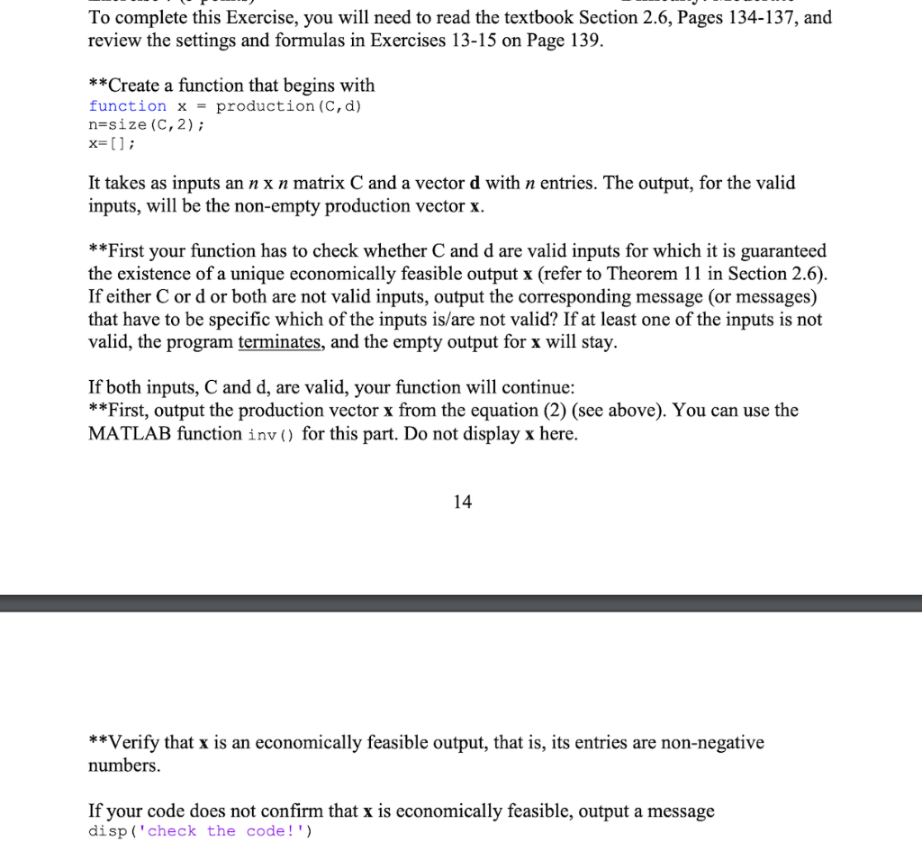
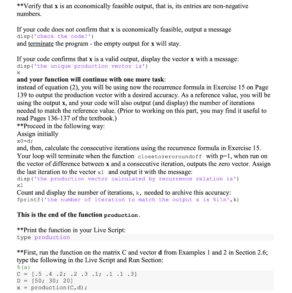
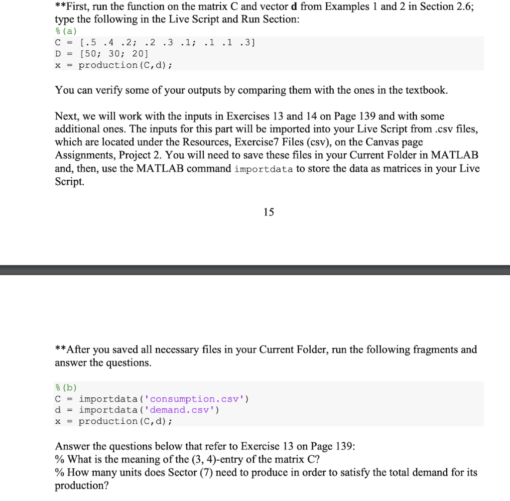
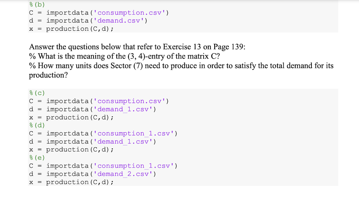
To complete this Exercise, you will need to read the textbook Section 2.6, Pages 134-137, and review the settings and formulas in Exercises 13-15 on Page 139. **Create a function that begins with function x = production (c,d) n=size (C, 2); x=[]; It takes as inputs an nx n matrix C and a vector d with n entries. The output, for the valid inputs, will be the non-empty production vector x. **First your function has to check whether C and d are valid inputs for which it is guaranteed the existence of a unique economically feasible output x (refer to Theorem 11 in Section 2.6). If either C or d or both are not valid inputs, output the corresponding message (or messages) that have to be specific which of the inputs is/are not valid? If at least one of the inputs is not valid, the program terminates, and the empty output for x will stay. If both inputs, C and d, are valid, your function will continue: **First, output the production vector x from the equation (2) (see above). You can use the MATLAB function inv() for this part. Do not display x here. 14 **Verify that x is an economically feasible output, that is, its entries are non-negative numbers. If your code does not confirm that x is economically feasible, output a message disp('check the code!') **Verify that x is an economically feasible output, that is, its entries are non-negative numbers. If your code does not confirm that x is economically feasible, output a message disp('check the code!') and terminate the program - the empty output for x will stay. If your code confirms that x is a valid output, display the vector x with a message: disp('the unique production vector is') x and your function will continue with one more task: instead of equation (2), you will be using now the recurrence formula in Exercise 15 on Page 139 to output the production vector with a desired accuracy. As a reference value, you will be using the output x, and your code will also output (and display) the number of iterations needed to match the reference value. (Prior to working on this part, you may find it useful to read Pages 136-137 of the textbook.) **Proceed in the following way: Assign initially x0=d; and, then, calculate the consecutive iterations using the recurrence formula in Exercise 15. Your loop will terminate when the function closetozeroroundoff with p=1, when run on the vector of difference between x and a consecutive iteration, outputs the zero vector. Assign the last iteration to the vector xl and output it with the message: disp('the production vector calculated by recurrence relation is') x1 Count and display the number of iterations, k, needed to archive this accuracy: fprintf('the number of iteration to match the output x is %i ',k) This is the end of the function production. **Print the function in your Live Script: type production **First, run the function on the matrix C and vector d from Examples 1 and 2 in Section 2.6; type the following in the Live Script and Run Section: % (a) [.5 .4 .2; .2 .3 .1; .1 .1 .3] D = [50; 30; 20) production (c,d); C = X = **First, run the function on the matrix C and vector d from Examples 1 and 2 in Section 2.6; type the following in the Live Script and Run Section: % (a) C = [.5 .4 .2; .2 .3 .1; .1 .1 .3] = [50; 30; 20] x = production (c,d); D You can verify some of your outputs by comparing them with the ones in the textbook. Next, we will work with the inputs in Exercises 13 and 14 on Page 139 and with some additional ones. The inputs for this part will be imported into your Live Script from .csv files, which are located under the Resources, Exercise7 Files (csv), on the Canvas page Assignments, Project 2. You will need to save these files in your Current Folder in MATLAB and, then, use the MATLAB command importdata to store the data as matrices in your Live Script. 15 **After you saved all necessary files in your Current Folder, run the following fragments and answer the questions. % (b) C = importdata ('consumption.csv') d = importdata ('demand.csv') X = production (c,d); Answer the questions below that refer to Exercise 13 on Page 139: % What is the meaning of the (3, 4)-entry of the matrix C? % How many units does Sector (7) need to produce in order to satisfy the total demand for its production? % (b) C = importdata ('consumption.csv') d importdata ('demand.csv') production (c,d); X = Answer the questions below that refer to Exercise 13 on Page 139: % What is the meaning of the (3, 4)-entry of the matrix C? % How many units does Sector (7) need to produce in order to satisfy the total demand for its production? = = (c) C = importdata('consumption.csv') d importdata ('demand 1.csv') X production (c,d); % (d) C importdata('consumption 1.csv') d = importdata ('demand_1.csv') x = production (c,d); % (e) C = importdata('consumption_1.csv') d = importdata ('demand_2.csv') production (C, d); X = 13. [M] The consumption matrix C below is based on input-output data for the U.S. economy in 1958, with data for 81 sectors grouped into 7 larger sectors: (1) nonmetal household and personal products, (2) final metal products (such as motor vehicles), (3) basic metal products and mining, (4) basic nonmetal products and agriculture, (5) energy, (6) services, and (7) entertainment and miscellaneous products. Find the production levels needed to satisfy the final demand d. (Units are in millions of dollars.) .1588 .0064 .0025 .0304 .0014 .0083 .1594 .0057 .2645 .0436 .0099 .0083 0201 3413 .0264 1506 3557.0139.0142 .0070 .0236 .3299 .0565 .0495 .3636 .0204 .0483 .0649 .0089 .0081 .0333 0295 3412.0237 .0020 .1190 0901.0996 .1260 .1722 .2368.3369 .0063 .0126 0196 .0098.0064.0132 .0012 74,000 56,000 10,500 d = 25,000 17,500 196,000 5,000 14. [M] The demand vector in Exercise 13 is reasonable for 1958 data, but Leontief's discussion of the economy in the reference cited there used a demand vector closer to 1964 data: d = (99640, 75548, 14444, 33501, 23527, 263985, 6526) Find the production levels needed to satisfy this demand. 15. [M] Use equation (6) to solve the problem in Exercise 13. Set x = d, and for k = 1, 2, ..., compute x(k) = d+ C x(k-1). How many steps are needed to obtain the answer in Exercise 13 to four significant figures? To complete this Exercise, you will need to read the textbook Section 2.6, Pages 134-137, and review the settings and formulas in Exercises 13-15 on Page 139. **Create a function that begins with function x = production (c,d) n=size (C, 2); x=[]; It takes as inputs an nx n matrix C and a vector d with n entries. The output, for the valid inputs, will be the non-empty production vector x. **First your function has to check whether C and d are valid inputs for which it is guaranteed the existence of a unique economically feasible output x (refer to Theorem 11 in Section 2.6). If either C or d or both are not valid inputs, output the corresponding message (or messages) that have to be specific which of the inputs is/are not valid? If at least one of the inputs is not valid, the program terminates, and the empty output for x will stay. If both inputs, C and d, are valid, your function will continue: **First, output the production vector x from the equation (2) (see above). You can use the MATLAB function inv() for this part. Do not display x here. 14 **Verify that x is an economically feasible output, that is, its entries are non-negative numbers. If your code does not confirm that x is economically feasible, output a message disp('check the code!') **Verify that x is an economically feasible output, that is, its entries are non-negative numbers. If your code does not confirm that x is economically feasible, output a message disp('check the code!') and terminate the program - the empty output for x will stay. If your code confirms that x is a valid output, display the vector x with a message: disp('the unique production vector is') x and your function will continue with one more task: instead of equation (2), you will be using now the recurrence formula in Exercise 15 on Page 139 to output the production vector with a desired accuracy. As a reference value, you will be using the output x, and your code will also output (and display) the number of iterations needed to match the reference value. (Prior to working on this part, you may find it useful to read Pages 136-137 of the textbook.) **Proceed in the following way: Assign initially x0=d; and, then, calculate the consecutive iterations using the recurrence formula in Exercise 15. Your loop will terminate when the function closetozeroroundoff with p=1, when run on the vector of difference between x and a consecutive iteration, outputs the zero vector. Assign the last iteration to the vector xl and output it with the message: disp('the production vector calculated by recurrence relation is') x1 Count and display the number of iterations, k, needed to archive this accuracy: fprintf('the number of iteration to match the output x is %i ',k) This is the end of the function production. **Print the function in your Live Script: type production **First, run the function on the matrix C and vector d from Examples 1 and 2 in Section 2.6; type the following in the Live Script and Run Section: % (a) [.5 .4 .2; .2 .3 .1; .1 .1 .3] D = [50; 30; 20) production (c,d); C = X = **First, run the function on the matrix C and vector d from Examples 1 and 2 in Section 2.6; type the following in the Live Script and Run Section: % (a) C = [.5 .4 .2; .2 .3 .1; .1 .1 .3] = [50; 30; 20] x = production (c,d); D You can verify some of your outputs by comparing them with the ones in the textbook. Next, we will work with the inputs in Exercises 13 and 14 on Page 139 and with some additional ones. The inputs for this part will be imported into your Live Script from .csv files, which are located under the Resources, Exercise7 Files (csv), on the Canvas page Assignments, Project 2. You will need to save these files in your Current Folder in MATLAB and, then, use the MATLAB command importdata to store the data as matrices in your Live Script. 15 **After you saved all necessary files in your Current Folder, run the following fragments and answer the questions. % (b) C = importdata ('consumption.csv') d = importdata ('demand.csv') X = production (c,d); Answer the questions below that refer to Exercise 13 on Page 139: % What is the meaning of the (3, 4)-entry of the matrix C? % How many units does Sector (7) need to produce in order to satisfy the total demand for its production? % (b) C = importdata ('consumption.csv') d importdata ('demand.csv') production (c,d); X = Answer the questions below that refer to Exercise 13 on Page 139: % What is the meaning of the (3, 4)-entry of the matrix C? % How many units does Sector (7) need to produce in order to satisfy the total demand for its production? = = (c) C = importdata('consumption.csv') d importdata ('demand 1.csv') X production (c,d); % (d) C importdata('consumption 1.csv') d = importdata ('demand_1.csv') x = production (c,d); % (e) C = importdata('consumption_1.csv') d = importdata ('demand_2.csv') production (C, d); X = 13. [M] The consumption matrix C below is based on input-output data for the U.S. economy in 1958, with data for 81 sectors grouped into 7 larger sectors: (1) nonmetal household and personal products, (2) final metal products (such as motor vehicles), (3) basic metal products and mining, (4) basic nonmetal products and agriculture, (5) energy, (6) services, and (7) entertainment and miscellaneous products. Find the production levels needed to satisfy the final demand d. (Units are in millions of dollars.) .1588 .0064 .0025 .0304 .0014 .0083 .1594 .0057 .2645 .0436 .0099 .0083 0201 3413 .0264 1506 3557.0139.0142 .0070 .0236 .3299 .0565 .0495 .3636 .0204 .0483 .0649 .0089 .0081 .0333 0295 3412.0237 .0020 .1190 0901.0996 .1260 .1722 .2368.3369 .0063 .0126 0196 .0098.0064.0132 .0012 74,000 56,000 10,500 d = 25,000 17,500 196,000 5,000 14. [M] The demand vector in Exercise 13 is reasonable for 1958 data, but Leontief's discussion of the economy in the reference cited there used a demand vector closer to 1964 data: d = (99640, 75548, 14444, 33501, 23527, 263985, 6526) Find the production levels needed to satisfy this demand. 15. [M] Use equation (6) to solve the problem in Exercise 13. Set x = d, and for k = 1, 2, ..., compute x(k) = d+ C x(k-1). How many steps are needed to obtain the answer in Exercise 13 to four significant figures