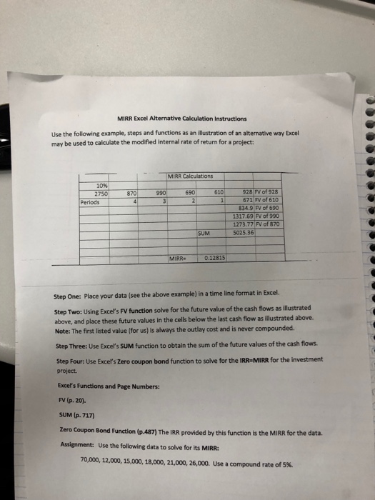
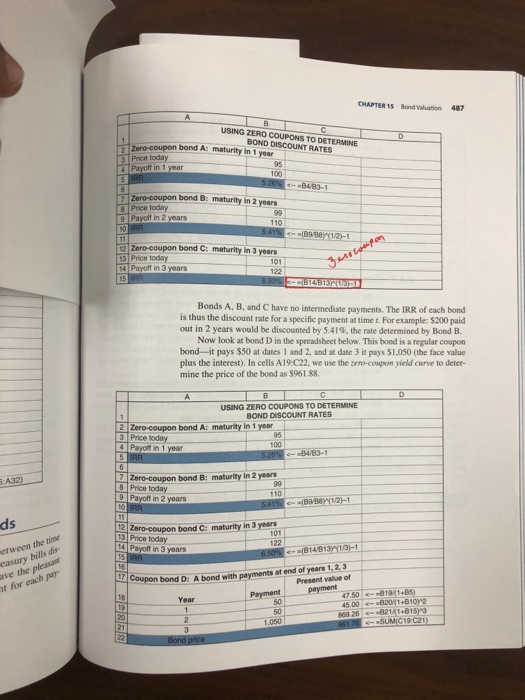
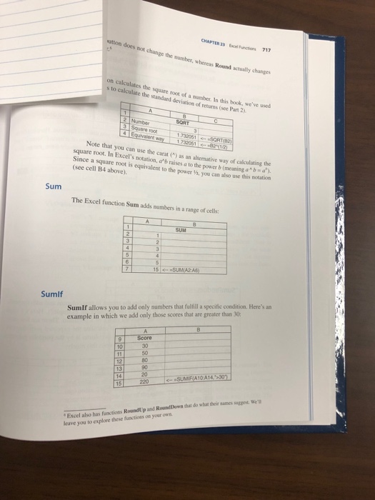
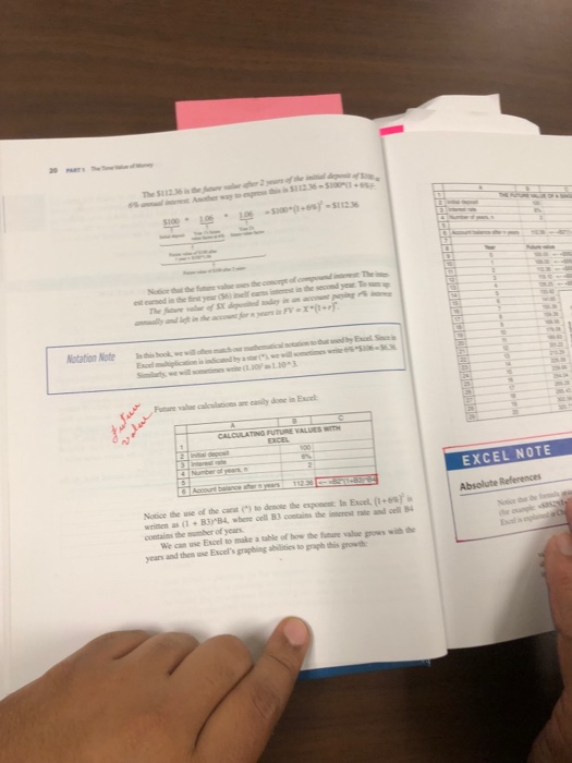
MIRR Excel Alternative Calculation Instructions Use the following example, steps and functions as an illustration of an alternative way Excel may be used to calculate the modified internal rate of return for a project: MIRR Calculations 1096 2750 928 FV of 928 671 FV of 610 834.9 FV of 690 1317.69 FV of 990 1273.77 FV of 870 870 990 690 610 Periods SUM 5025.36 MIRR- 0.12815 Step One: Place your data (see the above example) in a time line format in Excel. Step Two: Using Exce's FV function solve for the future value of the cash flows as llustrated above, and place these future values in the cells below the last cash flow as illustrated above. Note: The first listed value (for us) is always the outlay cost and is never compounded. Step Three: Use Excel's SUM function to obtain the sum of the future values of the cash flows Step Four: Use Excel's Zero coupon bond function to solve for the IRR-MIRR for the investment project Excel's Functions and Page Numbers: FV (p. 20). SUM (p. 717) Zero Coupon Bond Function (p.487) The IRR provided by this function is the MIRR for the data. Assignment: Use the following data to solve for its MIRR: 70,000, 12,000, 15, , 18,000, 21,000, 26,000, use a compound rate of 5%. MIRR Excel Alternative Calculation Instructions Use the following example, steps and functions as an illustration of an alternative way Excel may be used to calculate the modified internal rate of return for a project: MIRR Calculations 1096 2750 928 FV of 928 671 FV of 610 834.9 FV of 690 1317.69 FV of 990 1273.77 FV of 870 870 990 690 610 Periods SUM 5025.36 MIRR- 0.12815 Step One: Place your data (see the above example) in a time line format in Excel. Step Two: Using Exce's FV function solve for the future value of the cash flows as llustrated above, and place these future values in the cells below the last cash flow as illustrated above. Note: The first listed value (for us) is always the outlay cost and is never compounded. Step Three: Use Excel's SUM function to obtain the sum of the future values of the cash flows Step Four: Use Excel's Zero coupon bond function to solve for the IRR-MIRR for the investment project Excel's Functions and Page Numbers: FV (p. 20). SUM (p. 717) Zero Coupon Bond Function (p.487) The IRR provided by this function is the MIRR for the data. Assignment: Use the following data to solve for its MIRR: 70,000, 12,000, 15, , 18,000, 21,000, 26,000, use a compound rate of 5%
