Need help on this ASAP multiple linear regression question. see attached for data set
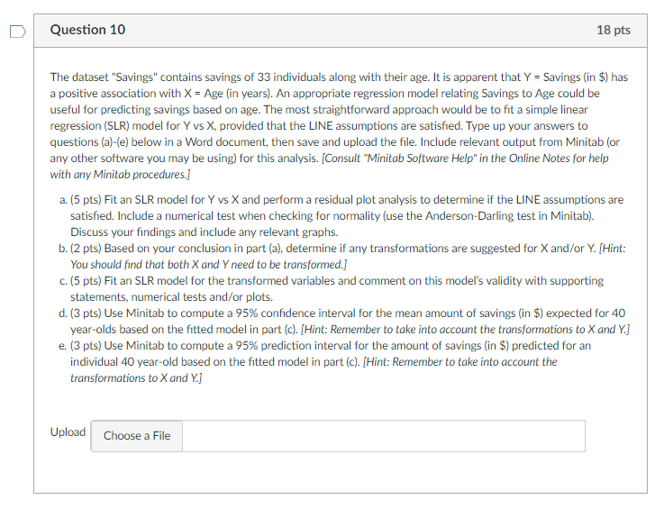
Question 1D The dataset "Savings" contains savings of 33 individuals along with their age. It is apparent that \"l" = Savings {in $} has a positive association with X = Age {in vears}. An appropriate regression model relating Savings to Age oould be useful for predicting savings based on age. The most straightforward approach would be to t a simple linear regression {SLR} model for '1" vs X, provided that the LINE assumptions are satised. Tvpe up 1vour answers to questions {ai-{el below in a Word document. then save and upload the le. Include relevant output from Minitab [or anv other software vou mav be using} for this analvsis. [Consult \"Mini tab Software Help" in the Dnline Notes for help with any Minitab procedures]1 a. {5 ptsi Fit an SLR model for v vs X and perform a residual plot analvsis to determine if the LINE assumptions are satised. Include a numerical test when checking for non'nalitv {use the Anderson'Da riing test in Minitab}. Discuss vour ndings and include anv relevant graphs. b. {2 ptsi Based on vour conclusion in part {a}. determine if anv transformations are suggested for X andr'or Y. IHint: "r'w should nd that both X and 'r need to be transformed} c. {5 ptsi Fit an SLR model for the transformed variables and comment on this model's validitv with supporting statements, numerical tests andr'or plots. d. {3 ptsi Use Minitab to compute a 95% condence interval for the mean amount of savings tin $1 expected for 4D 1vear-olds based on the tted model in part {c}. IHint: Remember to talce into account the transformations to 3K ana| "r'.]' e. {3 pts} Use Minitab to compute a 95% prediction interval for the amount of savings {in is} predicted for an individual 40 1rear-old based on the tted model in part [c]. IHint: Remember to take into accwnt the transformations to X and W Upload I Choose a File savings\tage 13728\t13 8062\t8 4805\t13 5099\t6 14963\t33 4295\t2 4046\t9 3193\t13 15486\t16 9413\t11 9034\t19 8939\t20 17596\t26 1884\t3 1763\t5 1233\t1 6286\t30 2849\t4 2818\t4 2265\t2 1652\t9 1846\t4 25460\t18 4570\t16 12213\t10 5870\t12 24484\t52 4735\t19 13334\t9 35381\t85 5681\t8 7161\t20 10592\t41 a. Test for Normal distribution of residuals Probability Plot of RESI1 Normal 99 Mean 3.307253E-13 StDev 4739 N 33 AD 0.919 P-Value 0.017 95 90 Percent 80 70 60 50 40 30 20 10 5 1 -10000 -5000 0 5000 10000 15000 RESI1 The AD p-value is grater than 0.05 which means that residual are not normally distributed or there is existence of an outlier. b. Fits and Diagnostics for Unusual Observations Obs 23 30 R X savings 25460 35381 Fit 9408 34351 Resid 16052 1030 Std Resid 3.39 0.32 R X Large residual Unusual X Observation 23 and 30 are outliers. c. Regression Analysis: savings versus age Method Rows unused 2 Analysis of Variance Source Regression age Error Lack-of-Fit Pure Error Total DF 1 1 29 18 11 30 Adj SS 494854488 494854488 446197911 229694091 216503820 941052399 Adj MS 494854488 494854488 15386135 12760783 19682165 F-Value 32.16 32.16 P-Value 0.000 0.000 0.65 0.800 Model Summary S 3922.52 R-sq 52.59% R-sq(adj) 50.95% R-sq(pred) 43.46% Coefficients Term Constant age Coef 2604 340.6 SE Coef 1103 60.1 T-Value 2.36 5.67 P-Value 0.025 0.000 VIF 1.00 Regression Equation savings = 2604 + 340.6 age Residual Plots for savings Normal Probability Plot Versus Fits 99 8000 Residual Percent 90 50 10 -5000 0 5000 0 -4000 -8000 10000 10000 15000 Fitted Value Histogram Versus Order 10.0 8000 7.5 4000 5.0 2.5 0.0 5000 Residual Residual Frequency 1 -10000 4000 -6000 -4000 -2000 0 2000 4000 6000 8000 20000 0 -4000 -8000 Residual The model is significant with a p-value less than 0.01. 1 5 10 15 20 Observation Order 25 30 From normality plot, residual are normally distributed since the plot is almost equal to a straight line. d. And Prediction for savings Regression Equation savings = 2604 + 340.6 age Variable age Fit 16227.8 Setting 40 SE Fit 1706.05 95% CI (12738.6, 19717.1) 95% PI (7479.42, 24976.2)