(Need help putting this question on excel. and what formulas to use)
Excel worksheet containing all four scenarios for JC Company (Exhibits 19.3 to 19.5)., it is required that you use formulas to calculate the values in all appropriate cells. In other words, you can only type in the aggregate production planning requirements once (see exhibit 19.3). Each subsequent time you use that information it should be through the use of a formula.
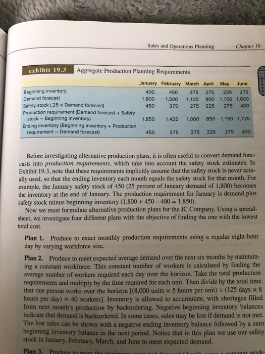
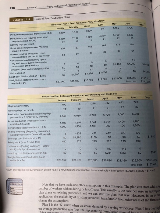
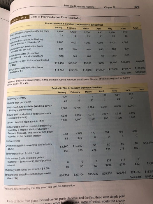
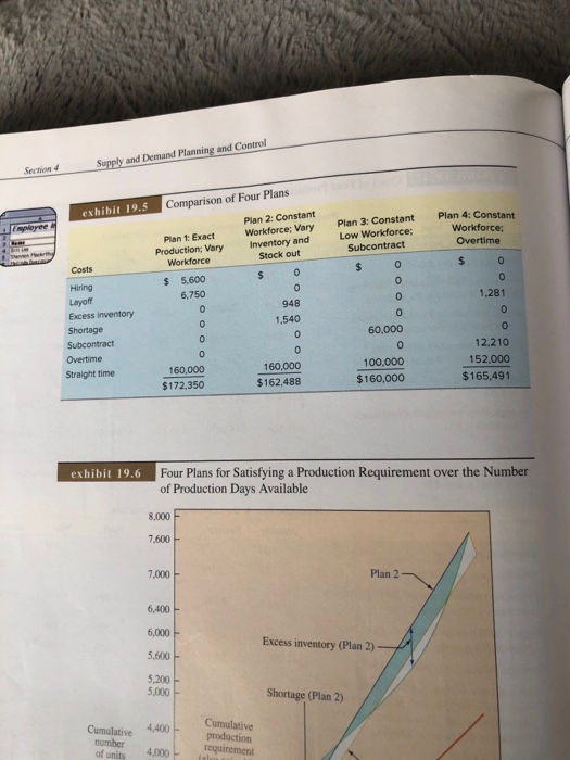
Sales and Operations Planning Chapter 19 exhibit 19.3 Aggregate Production Planning Requirements January February March April May 400 450 375 275 225 1,800 1.500 1.100 900 1,100 450 375 275 225 275 June 275 1,600 400 Beginning inventory Demand forecast Safety stock (25 x Demand forecast) Production requirement (Demand forecast + Safety stock - Beginning inventory) Ending inventory (Beginning inventory + Production requirement -Demand forecast) 1,850 450 1,425 375 1,000 275 850 225 1,150 1,725 275 400 Before investigating alternative production plans, it is often useful to convert demand fore- casts into production requirements, which take into account the safety stock estimates. In Exhibit 19.3, note that these requirements implicitly assume that the safety stock is never actu- ally used, so that the ending inventory each month equals the safety stock for that month. For example, the January safety stock of 450 (25 percent of January demand of 1,800) becomes the inventory at the end of January. The production requirement for January is demand plus safety stock minus beginning inventory (1,800 + 450 - 400 = 1.850). Now we must formulate alternative production plans for the JC Company. Using a spread- sheet, we investigate four different plans with the objective of finding the one with the lowest total cost. Plan 1. Produce to exact monthly production requirements using a regular eight-hour day by varying workforce size. Plan 2. Produce to meet expected average demand over the next six months by maintain ing a constant workforce. This constant number of workers is calculated by finding the average number of workers required each day over the horizon. Take the total production requirements and multiply by the time required for each unit. Then divide by the total time that one person works over the horizon [(8,000 units x 5 hours per unit) + (125 days X 8 hours per day) = 40 workers). Inventory is allowed to accumulate, with shortages filled from next month's production by backordering. Negative beginning inventory balances indicate that demand is backordered. In some cases, sales may be lost if demand is not met. The lost sales can be shown with a negative ending inventory balance followed by a zero beginning inventory balance in the next period. Notice that in this plan we use our safety stock in January, February, March, and June to meet expected demand. Plan 3. Produce to meet the constant work- Supply and Demand Planning and Control 498 Section 4 May 1,150 June 1.725 5.750 8.625 20 exhibit 19.4 Costs of Four Production Plans Production Plant Exact Productions Vary Workforce January February March April 850 Production requirement from Exhibit 193 1.850 1.425 1,000 Production hours required Production requirement x 5 hrunit) 4,250 7,125 9.250 5.000 Working days per month Hours per month per worker (Working days x Briday) Workers required Production hours required Hours per month per worken New workers hired assuming open. ing workforce equal to first month's requirement of 53 workers) Hiring cost New workers hired x $200) Workers laid off Layoff cost (Workers laid off x $250) $0 $1.500 $4,250 $1,000 Straight-time cost(Production hours required x $4) $37,000 $28.500 $20,000 $17.000 168 30 169 26 176 33 160 so 0 $0 $1,400 $4,200 55.600 O 56,750 $160.00 $172,350 $34,500 Total cost $23,000 22 1.600 Production Plan 2: Constant Workforce; Vary Inventory and Stock out January February March April May June Total Beginning inventory 400 8 -276 -32 412 720 19 21 Working days per month 22 0 21 20 Production hours available (Working days per month x 8 heday x 40 workers" 7,040 6,080 6,720 6,720 7,040 6,400 Actual production Production hours available/5 hrunit) 1.408 1,216 1,344 1,344 1.40B 1.280 Demand forecast from Exhibit 19.3) 1.800 1,500 1,100 900 1,100 Ending inventory (Beginning inventory+ Actual production-Demand forecast) 8 -276 -32 412 720 400 Shortage cost (Units short x $5) $0 $1,380 $160 $1.540 Safety stock (from Exhibit 19.3) 375 275 400 Units excess (Ending inventory - Safety stock) only if positive amount 187 445 Inventory cost (Units excess x $1.50) $0 $281 $668 $0 Straight-time cost Production hours $948 available x $4) $28,160 $24,320 $26,880 $26.880 $28,160 $25,600 $160.000 Total cost $162.488 Sum of production requirement in Exhibit 193 x 5htunity/Sum of production hours available he/day) = 18.000 x 5125 x B = 40 So $0 450 225 275 0 Note that we have made one other assumption in this example: The plan can start with number of workers with no hiring or layoff cost. This usually is the case because an aggregat plan draws on existing personnel, and we can start the plan that way. However, in an actus application, the availability of existing personnel transferable from other areas of the time change the assumptions. Plan 1 is the "S" curve when we chase demand by varying workforce. Plan 2 has the his est average production rate (the line representing cumulatiye demand has the Isinube Sales and Operations Planning Chapter 19 499 Costs of Four Production Plans (concluded) hibit 19.4 Production Plan 3: Constant Low Workforce Subcontract January February March April irement from Exhibit 19.3) 1.850 1425 1.000 850 22 21 Total May 1.150 22 June 1.725 20 con require jong days per month 4.400 3.800 4.200 4,200 4.400 4,000 880 760 840 840 880 800 on hours available (Working x iday x 25 workers) eduction Production hours wote 5hr per un subcontracted (Production wurement - Actual production) contracting cost (Units subcontracted * $20 httime cost(Production hours 970 665 160 10 270 925 $19.400 $13,300 $3200 200 $5,400 $18.500 500,000 $17.600 $15.200 $16.800 $16.800 lex 54) $17.600 $16,000 Total cost $100.000 $160.000 production requirement. In this example, Aprilis minimum of 850 units Number of workers required for Aprilis 350x57121x 8) - 25 Total May 554 22 June 792 200 6,688 6,080 1,338 1.100 1.216 1.600 Productio Plan 4: Constant Workforce Overtime January February March April Beginning inventory 4000 0 177 Working days per month 22 19 21 21 Production hours available (Working days x hriday x 38 workers" 6,688 5.776 6,384 6,384 Regular shift production (Production hours available/5 h/unit) 1,338 1,155 1.277 1.277 Demand forecast from Exhibit 19.3) 1,800 1,500 1,100 900 Units available before overtime (Beginning Inventory + Regular shift production - Demand forecast). This number has been -62 rounded to the nearest Integer. -345 177 554 Units overtime 62 375 0 0 Overtime cost (Units overtime x 5 hr/unit $6/hr.) $1,860 $10,350 Safety stock from Exhibit 19.3) 450 375 275 225 Units excess (Units available before overtime - Safety stock) only if positive 0 329 amount Inventory cost (Units excessive x $1.50) $494 Straight-time cost (Production hours avail- $26,752 523,104 $25,536 able x $4) $25.536 792 0 408 0 $12,210 $0 400 275 517 $776 $12 $1.28 $26,752 $24,320 Total cost $152.0 $165.4 Workers determined by trial and error. See text for explanation Each of these four plans focused on one particular cost, and the first three were simple pure m many other feasible plans, some of which would use a com- Supply and Demand Planning and Control Comparison of Four Plans exhibit 19.5 Plan 4: Constant Workforce; Overtime Plant Exact Production; Vary Workforce Plan 3: Constant Low Workforce; Subcontract $ 0 Plan 2: Constant Workforce: Vary Inventory and Stock out $ 0 Costs $ 5,600 6,750 1.281 948 1,540 Hiring Layoff Excess inventory Shortage Subcontract Overtime Straight time 60,000 12.210 152.000 $ 165,491 160,000 $172,350 100.000 $160,000 160,000 $162.488 exhibit 19.6 Four Plans for Satisfying a Production Requirement over the Number of Production Days Available 8,000 7.600 7.000 Plan 2 6,400 6,000 Excess inventory (Plan 2) 5.600 5.200 5.000 Shortage (Plan 2) 4400 Cumulative of units Cumulative production requirement number 4,000 Sales and Operations Planning Chapter 19 exhibit 19.3 Aggregate Production Planning Requirements January February March April May 400 450 375 275 225 1,800 1.500 1.100 900 1,100 450 375 275 225 275 June 275 1,600 400 Beginning inventory Demand forecast Safety stock (25 x Demand forecast) Production requirement (Demand forecast + Safety stock - Beginning inventory) Ending inventory (Beginning inventory + Production requirement -Demand forecast) 1,850 450 1,425 375 1,000 275 850 225 1,150 1,725 275 400 Before investigating alternative production plans, it is often useful to convert demand fore- casts into production requirements, which take into account the safety stock estimates. In Exhibit 19.3, note that these requirements implicitly assume that the safety stock is never actu- ally used, so that the ending inventory each month equals the safety stock for that month. For example, the January safety stock of 450 (25 percent of January demand of 1,800) becomes the inventory at the end of January. The production requirement for January is demand plus safety stock minus beginning inventory (1,800 + 450 - 400 = 1.850). Now we must formulate alternative production plans for the JC Company. Using a spread- sheet, we investigate four different plans with the objective of finding the one with the lowest total cost. Plan 1. Produce to exact monthly production requirements using a regular eight-hour day by varying workforce size. Plan 2. Produce to meet expected average demand over the next six months by maintain ing a constant workforce. This constant number of workers is calculated by finding the average number of workers required each day over the horizon. Take the total production requirements and multiply by the time required for each unit. Then divide by the total time that one person works over the horizon [(8,000 units x 5 hours per unit) + (125 days X 8 hours per day) = 40 workers). Inventory is allowed to accumulate, with shortages filled from next month's production by backordering. Negative beginning inventory balances indicate that demand is backordered. In some cases, sales may be lost if demand is not met. The lost sales can be shown with a negative ending inventory balance followed by a zero beginning inventory balance in the next period. Notice that in this plan we use our safety stock in January, February, March, and June to meet expected demand. Plan 3. Produce to meet the constant work- Supply and Demand Planning and Control 498 Section 4 May 1,150 June 1.725 5.750 8.625 20 exhibit 19.4 Costs of Four Production Plans Production Plant Exact Productions Vary Workforce January February March April 850 Production requirement from Exhibit 193 1.850 1.425 1,000 Production hours required Production requirement x 5 hrunit) 4,250 7,125 9.250 5.000 Working days per month Hours per month per worker (Working days x Briday) Workers required Production hours required Hours per month per worken New workers hired assuming open. ing workforce equal to first month's requirement of 53 workers) Hiring cost New workers hired x $200) Workers laid off Layoff cost (Workers laid off x $250) $0 $1.500 $4,250 $1,000 Straight-time cost(Production hours required x $4) $37,000 $28.500 $20,000 $17.000 168 30 169 26 176 33 160 so 0 $0 $1,400 $4,200 55.600 O 56,750 $160.00 $172,350 $34,500 Total cost $23,000 22 1.600 Production Plan 2: Constant Workforce; Vary Inventory and Stock out January February March April May June Total Beginning inventory 400 8 -276 -32 412 720 19 21 Working days per month 22 0 21 20 Production hours available (Working days per month x 8 heday x 40 workers" 7,040 6,080 6,720 6,720 7,040 6,400 Actual production Production hours available/5 hrunit) 1.408 1,216 1,344 1,344 1.40B 1.280 Demand forecast from Exhibit 19.3) 1.800 1,500 1,100 900 1,100 Ending inventory (Beginning inventory+ Actual production-Demand forecast) 8 -276 -32 412 720 400 Shortage cost (Units short x $5) $0 $1,380 $160 $1.540 Safety stock (from Exhibit 19.3) 375 275 400 Units excess (Ending inventory - Safety stock) only if positive amount 187 445 Inventory cost (Units excess x $1.50) $0 $281 $668 $0 Straight-time cost Production hours $948 available x $4) $28,160 $24,320 $26,880 $26.880 $28,160 $25,600 $160.000 Total cost $162.488 Sum of production requirement in Exhibit 193 x 5htunity/Sum of production hours available he/day) = 18.000 x 5125 x B = 40 So $0 450 225 275 0 Note that we have made one other assumption in this example: The plan can start with number of workers with no hiring or layoff cost. This usually is the case because an aggregat plan draws on existing personnel, and we can start the plan that way. However, in an actus application, the availability of existing personnel transferable from other areas of the time change the assumptions. Plan 1 is the "S" curve when we chase demand by varying workforce. Plan 2 has the his est average production rate (the line representing cumulatiye demand has the Isinube Sales and Operations Planning Chapter 19 499 Costs of Four Production Plans (concluded) hibit 19.4 Production Plan 3: Constant Low Workforce Subcontract January February March April irement from Exhibit 19.3) 1.850 1425 1.000 850 22 21 Total May 1.150 22 June 1.725 20 con require jong days per month 4.400 3.800 4.200 4,200 4.400 4,000 880 760 840 840 880 800 on hours available (Working x iday x 25 workers) eduction Production hours wote 5hr per un subcontracted (Production wurement - Actual production) contracting cost (Units subcontracted * $20 httime cost(Production hours 970 665 160 10 270 925 $19.400 $13,300 $3200 200 $5,400 $18.500 500,000 $17.600 $15.200 $16.800 $16.800 lex 54) $17.600 $16,000 Total cost $100.000 $160.000 production requirement. In this example, Aprilis minimum of 850 units Number of workers required for Aprilis 350x57121x 8) - 25 Total May 554 22 June 792 200 6,688 6,080 1,338 1.100 1.216 1.600 Productio Plan 4: Constant Workforce Overtime January February March April Beginning inventory 4000 0 177 Working days per month 22 19 21 21 Production hours available (Working days x hriday x 38 workers" 6,688 5.776 6,384 6,384 Regular shift production (Production hours available/5 h/unit) 1,338 1,155 1.277 1.277 Demand forecast from Exhibit 19.3) 1,800 1,500 1,100 900 Units available before overtime (Beginning Inventory + Regular shift production - Demand forecast). This number has been -62 rounded to the nearest Integer. -345 177 554 Units overtime 62 375 0 0 Overtime cost (Units overtime x 5 hr/unit $6/hr.) $1,860 $10,350 Safety stock from Exhibit 19.3) 450 375 275 225 Units excess (Units available before overtime - Safety stock) only if positive 0 329 amount Inventory cost (Units excessive x $1.50) $494 Straight-time cost (Production hours avail- $26,752 523,104 $25,536 able x $4) $25.536 792 0 408 0 $12,210 $0 400 275 517 $776 $12 $1.28 $26,752 $24,320 Total cost $152.0 $165.4 Workers determined by trial and error. See text for explanation Each of these four plans focused on one particular cost, and the first three were simple pure m many other feasible plans, some of which would use a com- Supply and Demand Planning and Control Comparison of Four Plans exhibit 19.5 Plan 4: Constant Workforce; Overtime Plant Exact Production; Vary Workforce Plan 3: Constant Low Workforce; Subcontract $ 0 Plan 2: Constant Workforce: Vary Inventory and Stock out $ 0 Costs $ 5,600 6,750 1.281 948 1,540 Hiring Layoff Excess inventory Shortage Subcontract Overtime Straight time 60,000 12.210 152.000 $ 165,491 160,000 $172,350 100.000 $160,000 160,000 $162.488 exhibit 19.6 Four Plans for Satisfying a Production Requirement over the Number of Production Days Available 8,000 7.600 7.000 Plan 2 6,400 6,000 Excess inventory (Plan 2) 5.600 5.200 5.000 Shortage (Plan 2) 4400 Cumulative of units Cumulative production requirement number 4,000