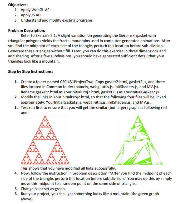
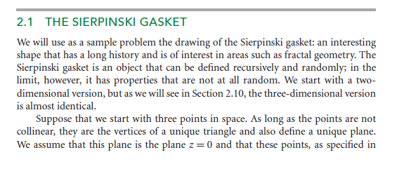
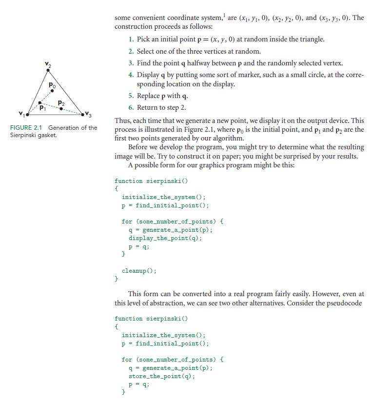
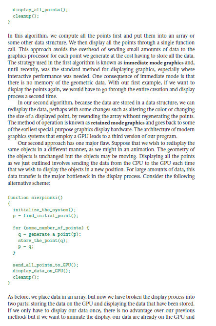
Objectives: 1. Apply WebGL API 2. Apply JS API 3. Understand and modify existing programs Problem Description: Refer to Exercise 2.1. A slight variation on generating the Sierpinski gasket with triangular polygons yields the fractal mountains used in computer-generated animations. After you find the midpoint of each side of the triangle, perturb this location before sub-division. Generate these triangles without fill. Later, you can do this exercise in three dimensions and add shading. After a few subdivisions, you should have generated sufficient detail that your triangles look like a mountain. Step by Step Instructions: 1. Create a folder named CSC1431Project Two. Copy gasket2.html, gasket2.js, and three files located in Common folder (namely, webgl-utils.js, initShaders.js, and MV.js). Rename gasket2.html as YourInitialProj2.html, gasket2.js as YourInitialGasket2.js. 2. Modify the links in YourInitialProj2.html, so that the following four files will be linked appropriately: YourInitialGasket2.js, webgl-utils.js, initShaders.js, and MV.js. 3. Test run first to ensure that you will get the similar (but larger) graph as following red one: AAAA This shows that you have modified all links successfully. 4. Now, follow the instruction in problem description: "After you find the midpoint of each side of the triangle, perturb this location before sub-division." You may do this by simply move this midpoint to a random point on the same side of triangle. 5. Change color set as green. 6. Run your project, you shall get something looks like a mountain (the green graph above). 2.1 THE SIERPINSKI GASKET We will use as a sample problem the drawing of the Sierpinski gasket: an interesting shape that has a long history and is of interest in areas such as fractal geometry. The Sierpinski gasket is an object that can be defined recursively and randomly; in the limit, however, it has properties that are not at all random. We start with a two- dimensional version, but as we will see in Section 2.10, the three-dimensional version is almost identical. Suppose that we start with three points in space. As long as the points are not collinear, they are the vertices of a unique triangle and also define a unique plane. We assume that this plane is the plane z=0 and that these points, as specified in some convenient coordinate system, are (X1, 1, 0), (X2, 72, 0), and (x3, 73, 0). The construction proceeds as follows: 1. Pick an initial point p=(x, y,0) at random inside the triangle. 2. Select one of the three vertices at random. 3. Find the point q halfway between p and the randomly selected vertex. 4. Display q by putting some sort of marker, such as a small circle, at the corre- sponding location on the display. 5. Replace p with q. 6. Return to step 2. Thus, each time that we generate a new point, we display it on the output device. This process is illustrated in Figure 2.1, where po is the initial point, and P, and P2 are the first two points generated by our algorithm. Before we develop the program, you might try to determine what the resulting image will be. Try to construct it on paper, you might be surprised by your results. A possible form for our graphics program might be this: FIGURE 2.1 Generation of the Sierpinski gasket. function sierpinski) initialize_the_system ; p = find_initial_point(); for (some_number_of_points) { q = generate_a_point(); display_the_point(); P = 9: cleanup(); This form can be converted into a real program fairly easily. However, even at this level of abstraction, we can see two other alternatives. Consider the pseudocode function sierpinski) initialize_the_system(); p = find initial_point(); for (some_number_of_points) { q = generate_a_point(p); store_the_point(); P = 9; display_all_points(): cleanup : In this algorithm, we compute all the points first and put them into an array or some other data structure. We then display all the points through a single function call. This approach avoids the overhead of sending small amounts of data to the graphics processor for each point we generate at the cost having to store all the data. The strategy used in the first algorithm is known as immediate mode graphics and, until recently, was the standard method for displaying graphics, especially where interactive performance was needed. One consequence of immediate mode is that there is no memory of the geometric data. With our first example, if we want to display the points again, we would have to go through the entire creation and display process a second time. In our second algorithm, because the data are stored in a data structure, we can redisplay the data, perhaps with some changes such as altering the color or changing the size of a displayed point, by resending the array without regenerating the points. The method of operation is known as retained mode graphics and goes back to some of the earliest special-purpose graphics display hardware. The architecture of modern graphics systems that employ a GPU leads to a third version of our program. Our second approach has one major flaw. Suppose that we wish to redisplay the same objects in a different manner, as we might in an animation. The geometry of the objects is unchanged but the objects may be moving. Displaying all the points as we just outlined involves sending the data from the CPU to the GPU each time that we wish to display the objects in a new position. For large amounts of data, this data transfer is the major bottleneck in the display process. Consider the following alternative scheme: function sierpinski initialize_the_system : P - find initial point: for (some_number_of_points) { 4-generate_a_point(p): store_the_point(): P-4: send_all_points_to_GPUO: display_data_on_GPUO: cleanup: As before, we place data in an array, but now we have broken the display process into two parts: storing the data on the GPU and displaying the data that have been stored. If we only have to display our data once, there is no advantage over our previous method; but if we want to animate the display, our data are already on the GPU and redisplay does not require any additional data transfer, only a simple function call that alters the location of some spatial data describing the objects that have moved. Although our final WebGL program will have a slightly different organization, we will follow this third strategy. We develop the full program in stages. First, we concentrate on the core: generating and displaying points. We must answer two questions: How do we represent points in space? Should we use two-dimensional, three-dimensional, or some other represen- tation? Once we answer these questions, we will be able to place our geometry on the GPU in a form that can be rendered. Then, we will be able to address how we view our objects using the power of programmable shaders. Objectives: 1. Apply WebGL API 2. Apply JS API 3. Understand and modify existing programs Problem Description: Refer to Exercise 2.1. A slight variation on generating the Sierpinski gasket with triangular polygons yields the fractal mountains used in computer-generated animations. After you find the midpoint of each side of the triangle, perturb this location before sub-division. Generate these triangles without fill. Later, you can do this exercise in three dimensions and add shading. After a few subdivisions, you should have generated sufficient detail that your triangles look like a mountain. Step by Step Instructions: 1. Create a folder named CSC1431Project Two. Copy gasket2.html, gasket2.js, and three files located in Common folder (namely, webgl-utils.js, initShaders.js, and MV.js). Rename gasket2.html as YourInitialProj2.html, gasket2.js as YourInitialGasket2.js. 2. Modify the links in YourInitialProj2.html, so that the following four files will be linked appropriately: YourInitialGasket2.js, webgl-utils.js, initShaders.js, and MV.js. 3. Test run first to ensure that you will get the similar (but larger) graph as following red one: AAAA This shows that you have modified all links successfully. 4. Now, follow the instruction in problem description: "After you find the midpoint of each side of the triangle, perturb this location before sub-division." You may do this by simply move this midpoint to a random point on the same side of triangle. 5. Change color set as green. 6. Run your project, you shall get something looks like a mountain (the green graph above). 2.1 THE SIERPINSKI GASKET We will use as a sample problem the drawing of the Sierpinski gasket: an interesting shape that has a long history and is of interest in areas such as fractal geometry. The Sierpinski gasket is an object that can be defined recursively and randomly; in the limit, however, it has properties that are not at all random. We start with a two- dimensional version, but as we will see in Section 2.10, the three-dimensional version is almost identical. Suppose that we start with three points in space. As long as the points are not collinear, they are the vertices of a unique triangle and also define a unique plane. We assume that this plane is the plane z=0 and that these points, as specified in some convenient coordinate system, are (X1, 1, 0), (X2, 72, 0), and (x3, 73, 0). The construction proceeds as follows: 1. Pick an initial point p=(x, y,0) at random inside the triangle. 2. Select one of the three vertices at random. 3. Find the point q halfway between p and the randomly selected vertex. 4. Display q by putting some sort of marker, such as a small circle, at the corre- sponding location on the display. 5. Replace p with q. 6. Return to step 2. Thus, each time that we generate a new point, we display it on the output device. This process is illustrated in Figure 2.1, where po is the initial point, and P, and P2 are the first two points generated by our algorithm. Before we develop the program, you might try to determine what the resulting image will be. Try to construct it on paper, you might be surprised by your results. A possible form for our graphics program might be this: FIGURE 2.1 Generation of the Sierpinski gasket. function sierpinski) initialize_the_system ; p = find_initial_point(); for (some_number_of_points) { q = generate_a_point(); display_the_point(); P = 9: cleanup(); This form can be converted into a real program fairly easily. However, even at this level of abstraction, we can see two other alternatives. Consider the pseudocode function sierpinski) initialize_the_system(); p = find initial_point(); for (some_number_of_points) { q = generate_a_point(p); store_the_point(); P = 9; display_all_points(): cleanup : In this algorithm, we compute all the points first and put them into an array or some other data structure. We then display all the points through a single function call. This approach avoids the overhead of sending small amounts of data to the graphics processor for each point we generate at the cost having to store all the data. The strategy used in the first algorithm is known as immediate mode graphics and, until recently, was the standard method for displaying graphics, especially where interactive performance was needed. One consequence of immediate mode is that there is no memory of the geometric data. With our first example, if we want to display the points again, we would have to go through the entire creation and display process a second time. In our second algorithm, because the data are stored in a data structure, we can redisplay the data, perhaps with some changes such as altering the color or changing the size of a displayed point, by resending the array without regenerating the points. The method of operation is known as retained mode graphics and goes back to some of the earliest special-purpose graphics display hardware. The architecture of modern graphics systems that employ a GPU leads to a third version of our program. Our second approach has one major flaw. Suppose that we wish to redisplay the same objects in a different manner, as we might in an animation. The geometry of the objects is unchanged but the objects may be moving. Displaying all the points as we just outlined involves sending the data from the CPU to the GPU each time that we wish to display the objects in a new position. For large amounts of data, this data transfer is the major bottleneck in the display process. Consider the following alternative scheme: function sierpinski initialize_the_system : P - find initial point: for (some_number_of_points) { 4-generate_a_point(p): store_the_point(): P-4: send_all_points_to_GPUO: display_data_on_GPUO: cleanup: As before, we place data in an array, but now we have broken the display process into two parts: storing the data on the GPU and displaying the data that have been stored. If we only have to display our data once, there is no advantage over our previous method; but if we want to animate the display, our data are already on the GPU and redisplay does not require any additional data transfer, only a simple function call that alters the location of some spatial data describing the objects that have moved. Although our final WebGL program will have a slightly different organization, we will follow this third strategy. We develop the full program in stages. First, we concentrate on the core: generating and displaying points. We must answer two questions: How do we represent points in space? Should we use two-dimensional, three-dimensional, or some other represen- tation? Once we answer these questions, we will be able to place our geometry on the GPU in a form that can be rendered. Then, we will be able to address how we view our objects using the power of programmable shaders