

Answered step by step
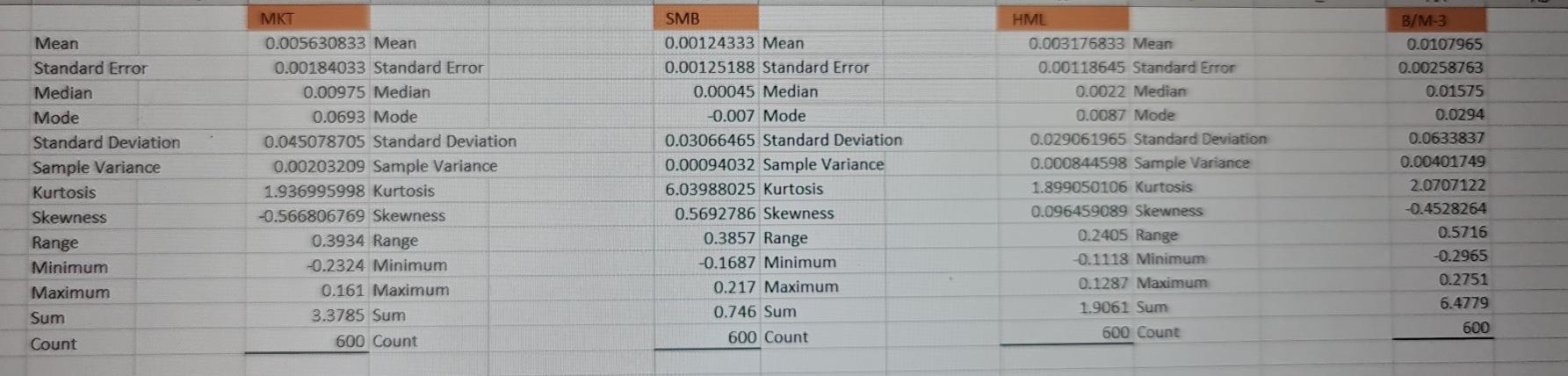
Verified Expert Solution
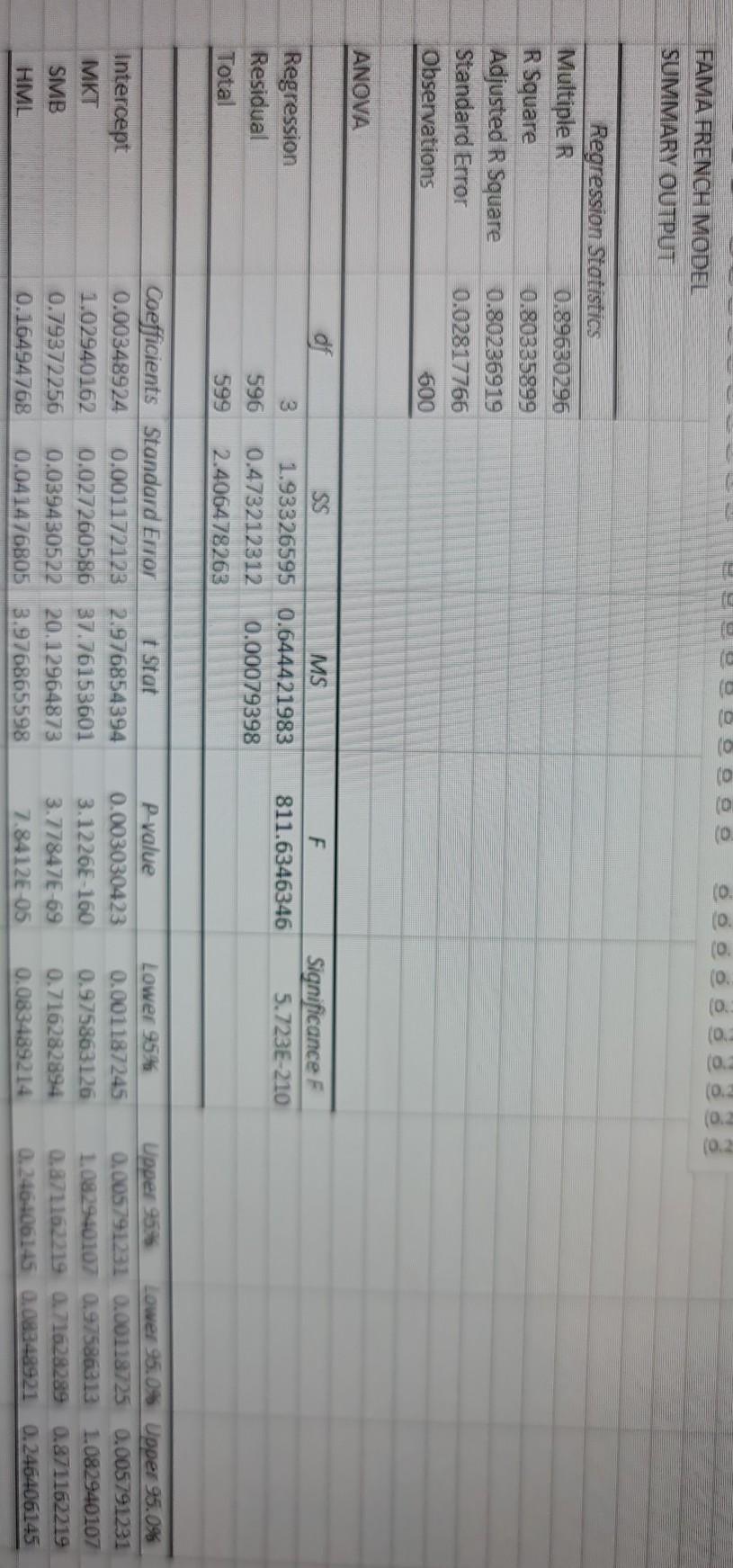
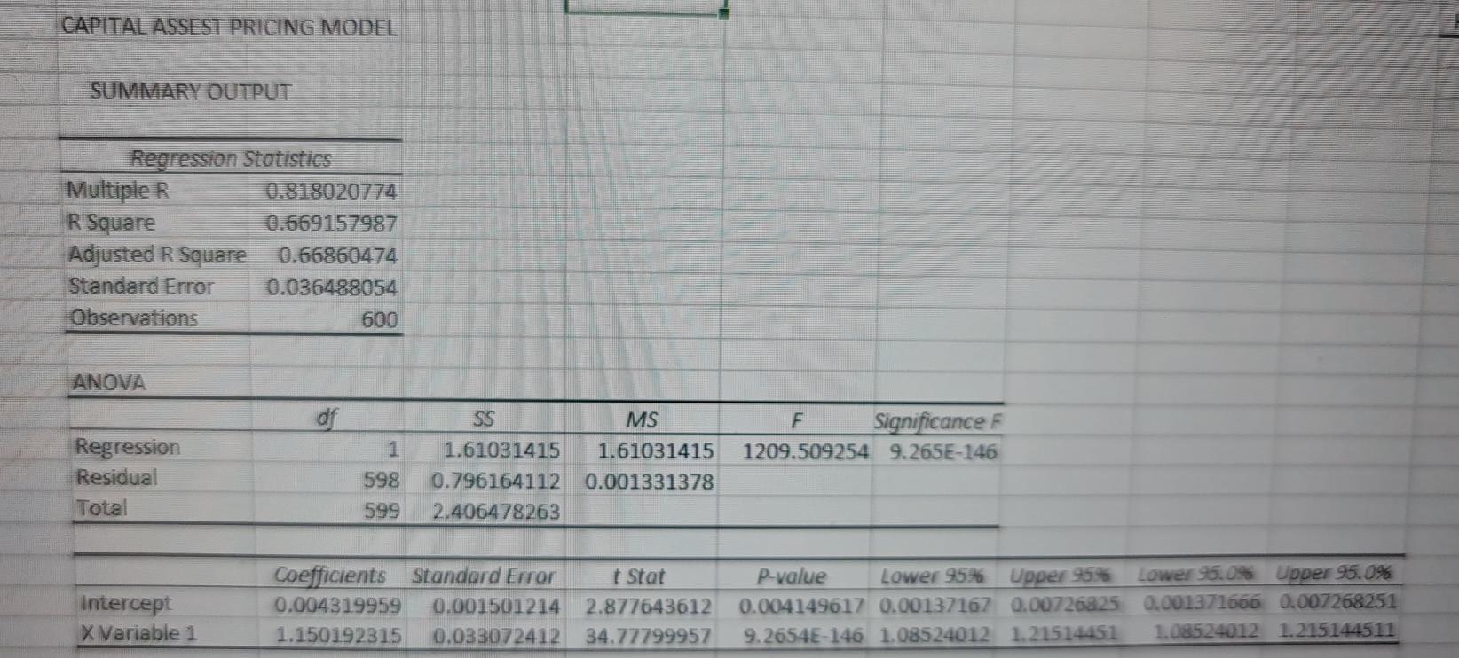
Question
1 Approved Answer
Old MathJax webview so b/m3 is portofolio, so for portfolio which model best suits it and explain why. and please tell how to calculate beta
Old MathJax webview


so b/m3 is portofolio, so for portfolio which model best suits it and explain why. and please tell how to calculate beta
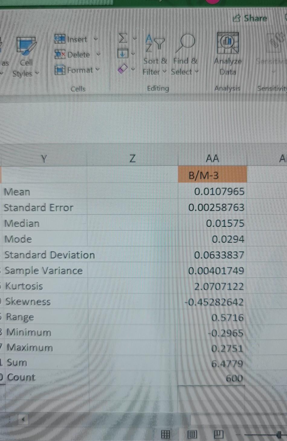
[1] Once you have been allocated your specific portfolio, you should begin by conducting a preliminary analysis of your time-series. To this end, you will need to compute and discuss some descriptive statistics of your portfolio's monthly returns. [2] You will then need to estimate two regression models. The first model is the Capital Asset Pricing Model (CAPM), and it is arguably the most widely known asset pricing model. The CAPM is given by the following equation R Re = a + BMKT; + &t where R, is the portfolio return at time t, MKT, denotes the return of the market at t, and & is a random error term. The second model is the Fama-French 3-factor model, another well-established asset pricing model, and it is given by the following equation Rt = a + B.MKT, + B2SMB, + B3 HML + et where the SMB factor refers to the returns of a portfolio of Small stocks minus the returns of a portfolio of Large stocks (in terms of market capitalization), and the HML factor refers to the returns of a portfolio of High-value stocks minus the 1 returns of a portfolio of Low-value stocks (in terms of book-to-market value). Once you have estimated the two regression models, you will need to discuss the empirical results in terms of intuition, statistical significance, goodness-of-fit etc. You will then need to run FULL diagnostic tests for each regression model, and discuss your results. Finally, you will need to compare the two models in terms of which one provides a more meaningful fit to your particular dataset. Mean Standard Error Median Mode Standard Deviation Sample Variance Kurtosis Skewness Range Minimum Maximum Sum Count MKT 0.005630833 Mean 0.00184033 Standard Error 0.00975 Median 0.0693 Mode 0.045078705 Standard Deviation 0.00203209 Sample Variance 1.936995998 kurtosis -0.566806769 Skewness 0.3934 Range -0.2324 Minimum 0.161 Maximum 3.3785 Sum 600 Count SMB 0.00124333 Mean 0.00125188 Standard Error 0.00045 Median -0.007 Mode 0.03066465 Standard Deviation 0.00094032 Sample Variance 6.03988025 Kurtosis 0.5692786 Skewness 0.3857 Range -0.1687 Minimum 0.217 Maximum 0.746 Sum 600 Count HML 0.003176833 Mean 0.00118645 Standard Error 0.0022 Median 0.0087 Mode 0.029061965 Standard Deviation 0.000844598 Sample Variance 1.899050106 Kurtosis 0.096459089 Skewness 0.2405 Range 0.1118 Minimum 0.1287 Maximum 1.9061 Sum B/M-3 0.0107965 0.00258763 0.01575 0.0294 0.0633837 0.00401749 2.0707122 -0.4528264 0.5716 -0.2965 0.2751 6.4779 600 600 Count (0. (0 (0. (0.3 FAMA FRENCH MODEL SUMMARY OUTPUT Regression Statistics Multiple R 0.89630296 R Square 0.80335899 Adjusted R Square 0.80236919 Standard Error 0.02817766 Observations 600 ANOVA df F 3 Significance F 5.723E-210 811.6346346 Regression Residual Total SS MS 1.93326595 0.644421983 0.473212312 0.00079398 2.406478263 596 599 Intercept MKT SMB HML Coefficients Standard Error t Stat 0.00348924 0.001172123 2.976854394 1.02940162 0.02726058637.76153601 0.79372256 0.039430522 20.12964873 0.16494768 0.041476805 3.976865598 P-value 0.003030423 3.1226E-160 3.77847E-69 7.8412E-05 Lower 95% 0.001187245 0.975863126 0.716282894 0.083489214 Upper 95% Lower 95.0% Upper 95.0% 0.005791231 0.00118725 0.005791231 1.082940107 0.975863131.082940107 0.871162219 0.71628289 0.871162219 0.246406145 0.08348921 0.246406145 CAPITAL ASSEST PRICING MODEL SUMMARY OUTPUT Regression Statistics Multiple R 0.818020774 R Square 0.669157987 Adjusted R Square 0.66860474 Standard Error 0.036488054 Observations 600 ANOVA df F Significance F 1209.509254 9.265E-146 Regression Residual Total SS 1.61031415 0.796164112 2.406478263 MS 1.61031415 0.001331378 598 599 Intercept X Variable 1 Coefficients Standard Error 0.004319959 0.001501214 1.150192315 0.033072412 t Stat 2.877643612 34.77799957 P-value Lower 95% Upper 95% 0.004149617 0.00137167 0.00726825 9.2654E-146 1.08524012 1.21514451 Lower 95.0% Upper 95.0% 0.001371666 0.007268251 1.08524012 1.215144511 3 Share Insert e B Delete as Cell Styles Sort & Find 8 Filter Select Analyze Data Format Cells Editing Analysis Sensitivit N A AA B/M-3 0.0107965 0.00258763 0.01575 0.0294 Mean Standard Error Median Mode Standard Deviation Sample Variance Kurtosis Skewness Range B Minimum Maximum 1 Sum Count 0.0633837 0.00401749 2.0707122 -0.45282642 0.5716 -0.2965 0.2751 6.4779 600 [1] Once you have been allocated your specific portfolio, you should begin by conducting a preliminary analysis of your time-series. To this end, you will need to compute and discuss some descriptive statistics of your portfolio's monthly returns. [2] You will then need to estimate two regression models. The first model is the Capital Asset Pricing Model (CAPM), and it is arguably the most widely known asset pricing model. The CAPM is given by the following equation R Re = a + BMKT; + &t where R, is the portfolio return at time t, MKT, denotes the return of the market at t, and & is a random error term. The second model is the Fama-French 3-factor model, another well-established asset pricing model, and it is given by the following equation Rt = a + B.MKT, + B2SMB, + B3 HML + et where the SMB factor refers to the returns of a portfolio of Small stocks minus the returns of a portfolio of Large stocks (in terms of market capitalization), and the HML factor refers to the returns of a portfolio of High-value stocks minus the 1 returns of a portfolio of Low-value stocks (in terms of book-to-market value). Once you have estimated the two regression models, you will need to discuss the empirical results in terms of intuition, statistical significance, goodness-of-fit etc. You will then need to run FULL diagnostic tests for each regression model, and discuss your results. Finally, you will need to compare the two models in terms of which one provides a more meaningful fit to your particular dataset. Mean Standard Error Median Mode Standard Deviation Sample Variance Kurtosis Skewness Range Minimum Maximum Sum Count MKT 0.005630833 Mean 0.00184033 Standard Error 0.00975 Median 0.0693 Mode 0.045078705 Standard Deviation 0.00203209 Sample Variance 1.936995998 kurtosis -0.566806769 Skewness 0.3934 Range -0.2324 Minimum 0.161 Maximum 3.3785 Sum 600 Count SMB 0.00124333 Mean 0.00125188 Standard Error 0.00045 Median -0.007 Mode 0.03066465 Standard Deviation 0.00094032 Sample Variance 6.03988025 Kurtosis 0.5692786 Skewness 0.3857 Range -0.1687 Minimum 0.217 Maximum 0.746 Sum 600 Count HML 0.003176833 Mean 0.00118645 Standard Error 0.0022 Median 0.0087 Mode 0.029061965 Standard Deviation 0.000844598 Sample Variance 1.899050106 Kurtosis 0.096459089 Skewness 0.2405 Range 0.1118 Minimum 0.1287 Maximum 1.9061 Sum B/M-3 0.0107965 0.00258763 0.01575 0.0294 0.0633837 0.00401749 2.0707122 -0.4528264 0.5716 -0.2965 0.2751 6.4779 600 600 Count (0. (0 (0. (0.3 FAMA FRENCH MODEL SUMMARY OUTPUT Regression Statistics Multiple R 0.89630296 R Square 0.80335899 Adjusted R Square 0.80236919 Standard Error 0.02817766 Observations 600 ANOVA df F 3 Significance F 5.723E-210 811.6346346 Regression Residual Total SS MS 1.93326595 0.644421983 0.473212312 0.00079398 2.406478263 596 599 Intercept MKT SMB HML Coefficients Standard Error t Stat 0.00348924 0.001172123 2.976854394 1.02940162 0.02726058637.76153601 0.79372256 0.039430522 20.12964873 0.16494768 0.041476805 3.976865598 P-value 0.003030423 3.1226E-160 3.77847E-69 7.8412E-05 Lower 95% 0.001187245 0.975863126 0.716282894 0.083489214 Upper 95% Lower 95.0% Upper 95.0% 0.005791231 0.00118725 0.005791231 1.082940107 0.975863131.082940107 0.871162219 0.71628289 0.871162219 0.246406145 0.08348921 0.246406145 CAPITAL ASSEST PRICING MODEL SUMMARY OUTPUT Regression Statistics Multiple R 0.818020774 R Square 0.669157987 Adjusted R Square 0.66860474 Standard Error 0.036488054 Observations 600 ANOVA df F Significance F 1209.509254 9.265E-146 Regression Residual Total SS 1.61031415 0.796164112 2.406478263 MS 1.61031415 0.001331378 598 599 Intercept X Variable 1 Coefficients Standard Error 0.004319959 0.001501214 1.150192315 0.033072412 t Stat 2.877643612 34.77799957 P-value Lower 95% Upper 95% 0.004149617 0.00137167 0.00726825 9.2654E-146 1.08524012 1.21514451 Lower 95.0% Upper 95.0% 0.001371666 0.007268251 1.08524012 1.215144511 3 Share Insert e B Delete as Cell Styles Sort & Find 8 Filter Select Analyze Data Format Cells Editing Analysis Sensitivit N A AA B/M-3 0.0107965 0.00258763 0.01575 0.0294 Mean Standard Error Median Mode Standard Deviation Sample Variance Kurtosis Skewness Range B Minimum Maximum 1 Sum Count 0.0633837 0.00401749 2.0707122 -0.45282642 0.5716 -0.2965 0.2751 6.4779 600
Step by Step Solution
There are 3 Steps involved in it
Step: 1

Get Instant Access to Expert-Tailored Solutions
See step-by-step solutions with expert insights and AI powered tools for academic success
Step: 2

Step: 3
Ace Your Homework with AI
Get the answers you need in no time with our AI-driven, step-by-step assistance
Get Started
Cryptocurrency QuickStart Guide
Authors: Jonathan Reichental
1st Edition
1636100406, 978-1636100401