

Answered step by step
Verified Expert Solution
Question
1 Approved Answer
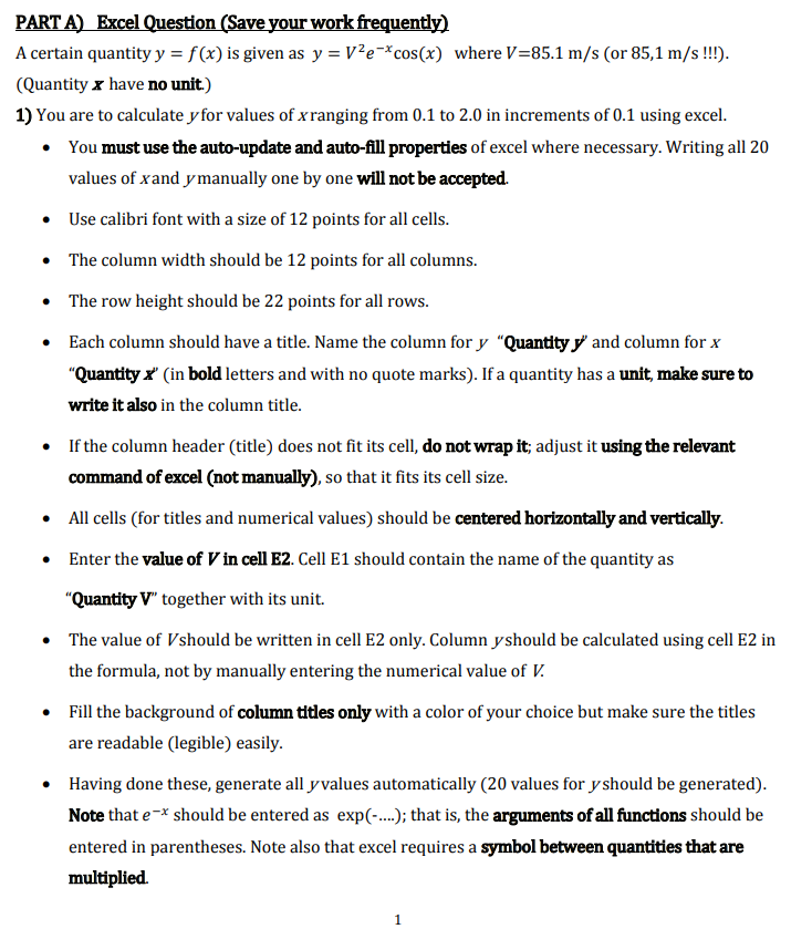
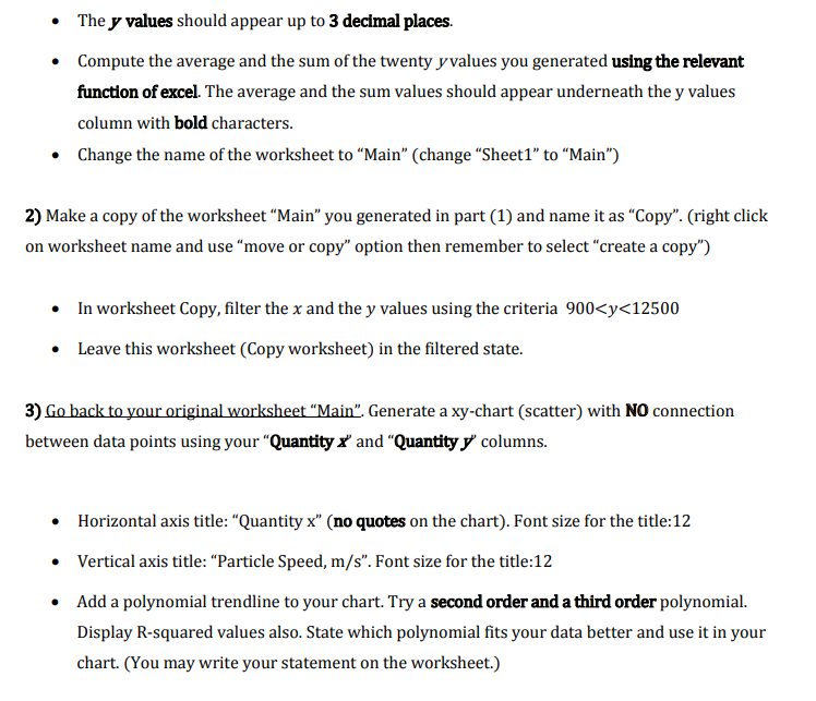
PART A) Excel Question (Save your work frequently) A certain quantity y = f(x) is given as y = V2e-*cos(x) where V=85.1 m/s (or 85,1
Step by Step Solution
There are 3 Steps involved in it
Step: 1

Get Instant Access to Expert-Tailored Solutions
See step-by-step solutions with expert insights and AI powered tools for academic success
Step: 2

Step: 3
Ace Your Homework with AI
Get the answers you need in no time with our AI-driven, step-by-step assistance
Get Started
The Language Of Influence And Personal Power
Authors: Scott Hagan
1st Edition
1944833560, 978-1944833565