

Question: please answer part c and part d only. do not hard-code show me the functions A A B C D E F F Module 13.
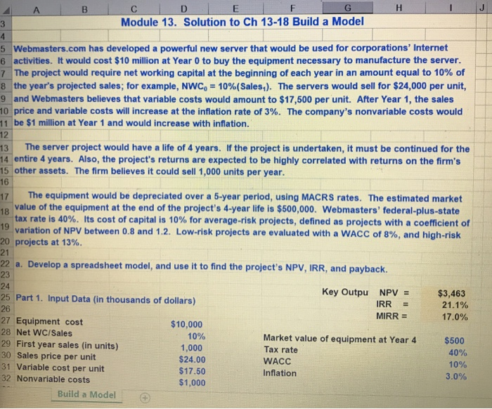
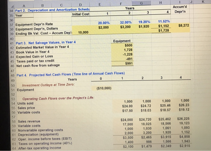
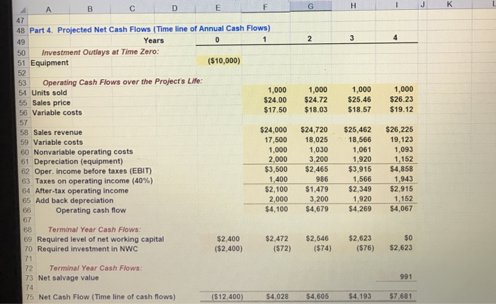
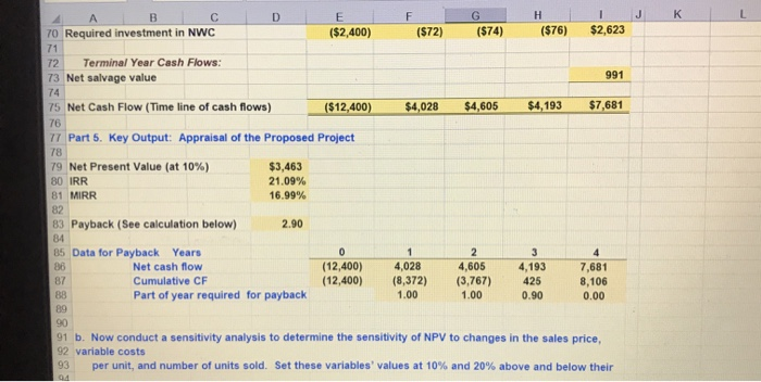
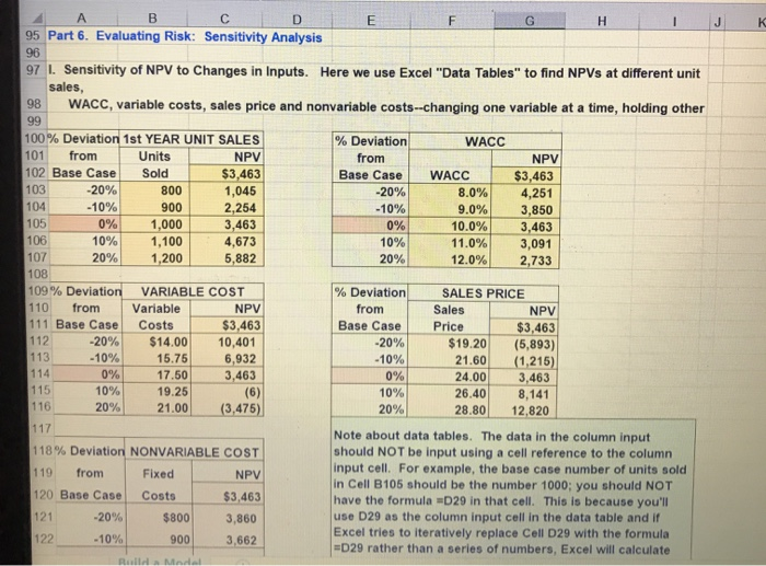
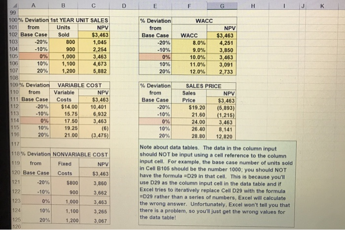
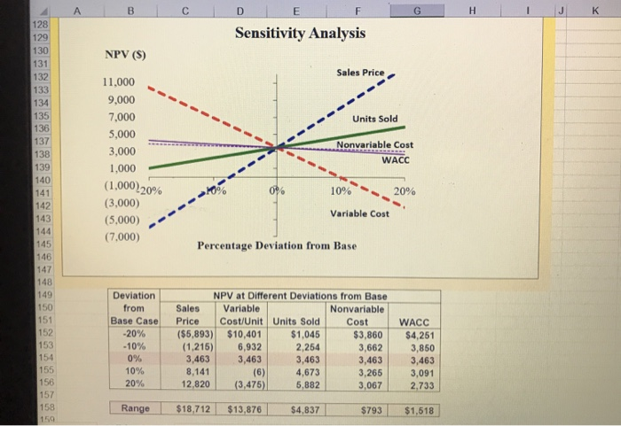
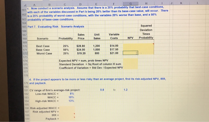
A A B C D E F F Module 13. Solution to Ch 13-18 Build a Model w 5 Webmasters.com has developed a powerful new server that would be used for corporations' Internet 6 activities. It would cost $10 million at Year 0 to buy the equipment necessary to manufacture the server. 7 The project would require net working capital at the beginning of each year in an amount equal to 10% of 8 the year's projected sales, for example, NWC, = 10%(Sales). The servers would sell for $24,000 per unit, 9 and Webmasters believes that variable costs would amount to $17,500 per unit. After Year 1, the sales 10 price and variable costs will increase at the inflation rate of 3%. The company's nonvariable costs would 11 be $1 million at Year 1 and would increase with inflation. 13 The server project would have a life of 4 years. If the project is undertaken, it must be continued for the 14 entire 4 years. Also, the project's returns are expected to be highly correlated with returns on the firm's 15 other assets. The firm believes it could sell 1,000 units per year. 16 17 The equipment would be depreciated over a 5-year period, using MACRS rates. The estimated market o value of the equipment at the end of the project's 4-year life is $500,000. Webmasters' federal-plus-state tax rate is 40%. Its cost of capital is 10% for average-risk projects, defined as projects with a coefficient of 19 variation of NPV between 0.8 and 1.2. Low-risk projects are evaluated with a WACC of 8%, and high-risk 20 projects at 13%. 22 a. Develop a spreadsheet model, and use it to find the project's NPV, IRR, and payback. 24 25 Part 1. Input Data (in thousands of dollars) 26 Key Outpu NPV = IRR = MIRR = $3,463 21.1% 17.0% 27 Equipment cost 28 Net WC/Sales 29 First year sales (in units) 30 Sales price per unit 31 Variable cost per unit 32 Nonvariable costs Build a Model $10,000 10% 1,000 $24.00 $17.50 $1,000 Market value of equipment at Year 4 Tax rate WACC Inflation $500 40% 10% 3.0% GHIJK Years Accum'd 2 3 4 Depr'n 20.00% $2,000 32.00% $3,200 19.20% $1,920 11.52% $1,152 $1,728 $8,272 LA BC D 34 Part 2. Depreciation and Amortization Schedu 35 Year Initial Cost 36 37 Equipment Depr'n Rate 38 Equipment Depr'n, Dollars 39 Ending Bk Val: Cost - Accum Dep'i 10,000 40 41 Part 3. Net Salvage Values, in Year 4 42 Estimated Market Value in Year 4 43 Book Value in Year 4 44 Expected Gain or Loss 45 Taxes paid or tax credit 46 Net cash flow from salvage Equipment $500 1.728 -1,228 -491 $991 48 Part 4. Projected Net Cash Flows (Time line of Annual Cash Flows) Years 50 Investment Outlays at Time Zero: 51 Equipment ($10,000) 53 Operating Cash Flows over the Project's Life: 54 Units sold 55 Sales price 56 Variable costs 1,000 $24.00 $17.50 1,000 $24.72 $18.03 1,000 $25.46 $18.57 1,000 $26.23 $19.12 57 58 Sales revenue 59 Variable costs 60 Nonvariable operating costs 61 Depreciation (equipment) 62 Oper. Income before taxes (EBIT) 63 Taxes on operating income (40%) 64 After-tax operating income $24,000 17,500 1,000 2,000 $3,500 1,400 $2,100 $24,720 18,025 1,030 3,200 $2,465 986 $1,479 $25,462 18,566 1,061 1,920 $3,915 1,566 $2,349 $26,225 19,123 1,093 1,152 $4,858 1,943 $2,915 B C D E 48 Part 4. Projected Net Cash Flows (Time line of Annual Cash Flows) Years 50 Investment Outlays at Time Zero: 51 Equipment ($10,000) 53 Operating Cash Flows over the Project's Life: 54 Units sold 55 Sales price 56 Variable costs 1,000 $24.00 $17.50 1,000 $24.72 $18.03 1,000 $25.46 $18.57 1,000 $26.23 $19.12 58 Sales revenue 59 Variable costs 60 Nonvariable operating costs 61 Depreciation (equipment) 62 Oper income before taxes (EBIT) 63 Taxes on operating income (40%) 64 After-tax operating income 65 Add back depreciation 66 Operating cash flow $24,000 17,500 1,000 2,000 $3,500 1,400 $2,100 2.000 $4,100 $24,720 18,025 1,030 3,200 $2,465 986 $1,479 3,200 $4,679 $25,462 18,566 1,061 1,920 $3,915 1,566 $2,349 1,920 $4,269 $26,225 19,123 1,093 1,152 $4,858 1,943 $2.915 1,152 $4,067 68 Terminal Year Cash Flows: 69 Required level of net working capital 70 Required investment in NWC $0 $2,400 ($2,400) $2,472 (572) $2,546 ($74) $2,623 (576) $2,623 72 Terminal Year Cash Flows: 73 Net salvage value 991 75 Net Cash Flow (Time line of cash flows) ($12,400) $4.028 $4.605 $4.193 $7,681 J K A B C 70 Required investment in NWC E ($2,400) o (872) G ($74) H ($76) I $2,623 72 Terminal Year Cash Flows: 73 Net salvage value 991 75 Net Cash Flow (Time line of cash flows) ($12,400) $4,028 $4,605 $4,193 $7,681 76 IT Part 5. Key Output: Appraisal of the Proposed Project 78 79 Net Present Value (at 10%) 80 IRR 81 MIRR $3,463 21.09% 16.99% 83 Payback (See calculation below) 2.90 85 Data for Payback Years Net cash flow Cumulative CF Part of year required for payback (12,400) (12,400) 4,028 (8,372) 1.00 4,605 (3,767) 1.00 4,193 425 0.90 7,681 8,106 0.00 91 b. Now conduct a sensitivity analysis to determine the sensitivity of NPV to changes in the sales price, 92 variable costs 93 per unit, and number of units sold. Set these variables' values at 10% and 20% above and below their H 4 ABC 95 Part 6. Evaluating Risk: Sensitivity Analysis 105 97 I. Sensitivity of NPV to Changes in Inputs. Here we use Excel "Data Tables" to find NPVs at different unit sales, 98 WACC, variable costs, sales price and nonvariable costs--changing one variable at a time, holding other 99 100% Deviation 1st YEAR UNIT SALES % Deviation WACC 101 from Units NPV from NPV 102 Base Case Sold $3,463 Base Case WACC $3,463 103 -20% 800 1,045 -20% 8.0% 4,251 104 -10% 900 2,254 -10% 9.0% 3,850 0% 1,000 3,463 0% 10.0% 3,463 106 10% 1,100 4,673 10% 11.0% 3,091 107 20% 1,200 5,882 20% 12.0% 2,733 108 109 % Deviation VARIABLE COST % Deviation SALES PRICE 110 from Variable NPV from Sales NPV 111 Base Case Costs $3,463 Base Case Price $3,463 112 -20% $14.00 10,401 -20% $19.20 (5,893) 113 -10% 15.75 6,932 -10% 21.60 (1,215) 114 0% 17.50 3,463 0% 24.00 3,463 115 19.25 (6) 10% 26.408,141 116 20% 21.00 (3,475) 20% 28.80 12,820 117 Note about data tables. The data in the column input 118% Deviation NONVARIABLE COST should NOT be input using a cell reference to the column 119 from Fixed NPV input cell. For example, the base case number of units sold in Cell B105 should be the number 1000; you should NOT 120 Base Case Costs $3,463 have the formula D29 in that cell. This is because you'll 121 -20% $800 3,860 use D29 as the column input cell in the data table and if Excel tries to iteratively replace Cell D29 with the formula 122 - 10% 900 3,662 -D29 rather than a series of numbers, Excel will calculate 10% AB G JK 99 WACC 100% Deviation 1st YEAR UNIT SALES from Units NPV 102 Base Case Sold $3,463 -20% 800 1,045 -10% 900 2,254 0% 1,000 3,463 10% 1,100 4,673 20% 1,200 5,882 % Deviation from Base Case -20% -10% 0% 10% 20% WACC 8.0% 9.0% 10.0% 11.0% 12.0% NPV $3,463 4,251 3,850 3,463 3,091 2,733 % Deviation from Base Case -20% -10% 0% 10% 20% SALES PRICE Sales NPV Price $3,463 $19.20 (5,893) 21.60 (1,215) 24.00 3,463 26.408 ,141 28.80 12,820 0% (6) 109 % Deviation VARIABLE COST 110 from NPV 111 Base Case Costs $3,463 112 -20% $14.00 10,401 113 -10% 15.75 6,932 114 17.50 3,463 115 10% 19.25 116 20% 21.00 (3,475) 117 118% Deviation NONVARIABLE COST 119 from Fixed NPV 120 Base Case Costs $3,463 -20% $800 3,860 - 10% 900 3,662 0% 1,000 3,463 10% 1,100 3,265 20% 1,200 3,067 Note about data tables. The data in the column input should NOT be input using a cell reference to the column input cell. For example, the base case number of units sold in Cell B105 should be the number 1000; you should NOT have the formula =D29 in that cell. This is because you'll use D29 as the column input cell in the data table and if Excel tries to iteratively replace Cell D29 with the formula =D29 rather than a series of numbers, Excel will calculate the wrong answer. Unfortunately, Excel won't tell you that there is a problem, so you'll just get the wrong values for the data table! A B C DF D Sensitivity Analysis NPV (S) Sales Price Units Sold 11,000 9,000 7,000 5,000 3,000 1,000 Nonvariable Cost WACC (1.000 20% 10% 20% Variable Cost (3,000) (5,000) (7.000) Percentage Deviation from Base Deviation from Base Case -20% -10% 0% 10% 20% NPV at Different Deviations from Base Sales Variable Nonvariable Cost/Unit Units Sold Cost ($5,893) $10,401 $1,045 $3,860 (1,215) 6,932 2,254 3,662 3,463 3,463 3,463 3,463 8,141 4,673 3,265 12,820 (3,475) 5,882 3,067 WACC $4,251 3,850 3,463 3,091 2.733 155 (6) 156 157 158 Range $18,712 $13,876 $4,837 $793 $1,618 J K L A B C D E F G H I c. Now conduct a scenario analysis. Assume that there is a 25% probability that best-case conditions, with each of the variables discussed in Part b being 20% better than its base-case value, will occur. There 102 is a 25% probability of worst-case conditions, with the variables 20% worse than base, and a 50% 163 probability of base-case conditions 165 Part 7. Evaluating Risk: Scenario Analysis 166 Squared Deviation Times Probability 168 Probability Sales Price Unit Sales Variable Costs NPV 169 170 Best Case Base Case Worst Case 25% 50% 25% $28.80 $24.00 $19.20 1,200 1,000 800 $14.00 $17.50 $21.00 174 175 Expected NPV = sum, prob times NPV Standard Deviation - Sq Root of column H sum Coefficient of Variation - Std Dev / Expected NPV 178 d. If the project appears to be more or less risky than an average project, find its risk-adjusted NPV, IRR, 179 and payback 180 181 CV range of firm's average-risk project: 182 Low-risk WACC 89% 183 WACC 10 184 High-risk WACC 105 186 Risk-adjusted WACC 187 Risk adjusted NPV IRR Payback 13% A A B C D E F F Module 13. Solution to Ch 13-18 Build a Model w 5 Webmasters.com has developed a powerful new server that would be used for corporations' Internet 6 activities. It would cost $10 million at Year 0 to buy the equipment necessary to manufacture the server. 7 The project would require net working capital at the beginning of each year in an amount equal to 10% of 8 the year's projected sales, for example, NWC, = 10%(Sales). The servers would sell for $24,000 per unit, 9 and Webmasters believes that variable costs would amount to $17,500 per unit. After Year 1, the sales 10 price and variable costs will increase at the inflation rate of 3%. The company's nonvariable costs would 11 be $1 million at Year 1 and would increase with inflation. 13 The server project would have a life of 4 years. If the project is undertaken, it must be continued for the 14 entire 4 years. Also, the project's returns are expected to be highly correlated with returns on the firm's 15 other assets. The firm believes it could sell 1,000 units per year. 16 17 The equipment would be depreciated over a 5-year period, using MACRS rates. The estimated market o value of the equipment at the end of the project's 4-year life is $500,000. Webmasters' federal-plus-state tax rate is 40%. Its cost of capital is 10% for average-risk projects, defined as projects with a coefficient of 19 variation of NPV between 0.8 and 1.2. Low-risk projects are evaluated with a WACC of 8%, and high-risk 20 projects at 13%. 22 a. Develop a spreadsheet model, and use it to find the project's NPV, IRR, and payback. 24 25 Part 1. Input Data (in thousands of dollars) 26 Key Outpu NPV = IRR = MIRR = $3,463 21.1% 17.0% 27 Equipment cost 28 Net WC/Sales 29 First year sales (in units) 30 Sales price per unit 31 Variable cost per unit 32 Nonvariable costs Build a Model $10,000 10% 1,000 $24.00 $17.50 $1,000 Market value of equipment at Year 4 Tax rate WACC Inflation $500 40% 10% 3.0% GHIJK Years Accum'd 2 3 4 Depr'n 20.00% $2,000 32.00% $3,200 19.20% $1,920 11.52% $1,152 $1,728 $8,272 LA BC D 34 Part 2. Depreciation and Amortization Schedu 35 Year Initial Cost 36 37 Equipment Depr'n Rate 38 Equipment Depr'n, Dollars 39 Ending Bk Val: Cost - Accum Dep'i 10,000 40 41 Part 3. Net Salvage Values, in Year 4 42 Estimated Market Value in Year 4 43 Book Value in Year 4 44 Expected Gain or Loss 45 Taxes paid or tax credit 46 Net cash flow from salvage Equipment $500 1.728 -1,228 -491 $991 48 Part 4. Projected Net Cash Flows (Time line of Annual Cash Flows) Years 50 Investment Outlays at Time Zero: 51 Equipment ($10,000) 53 Operating Cash Flows over the Project's Life: 54 Units sold 55 Sales price 56 Variable costs 1,000 $24.00 $17.50 1,000 $24.72 $18.03 1,000 $25.46 $18.57 1,000 $26.23 $19.12 57 58 Sales revenue 59 Variable costs 60 Nonvariable operating costs 61 Depreciation (equipment) 62 Oper. Income before taxes (EBIT) 63 Taxes on operating income (40%) 64 After-tax operating income $24,000 17,500 1,000 2,000 $3,500 1,400 $2,100 $24,720 18,025 1,030 3,200 $2,465 986 $1,479 $25,462 18,566 1,061 1,920 $3,915 1,566 $2,349 $26,225 19,123 1,093 1,152 $4,858 1,943 $2,915 B C D E 48 Part 4. Projected Net Cash Flows (Time line of Annual Cash Flows) Years 50 Investment Outlays at Time Zero: 51 Equipment ($10,000) 53 Operating Cash Flows over the Project's Life: 54 Units sold 55 Sales price 56 Variable costs 1,000 $24.00 $17.50 1,000 $24.72 $18.03 1,000 $25.46 $18.57 1,000 $26.23 $19.12 58 Sales revenue 59 Variable costs 60 Nonvariable operating costs 61 Depreciation (equipment) 62 Oper income before taxes (EBIT) 63 Taxes on operating income (40%) 64 After-tax operating income 65 Add back depreciation 66 Operating cash flow $24,000 17,500 1,000 2,000 $3,500 1,400 $2,100 2.000 $4,100 $24,720 18,025 1,030 3,200 $2,465 986 $1,479 3,200 $4,679 $25,462 18,566 1,061 1,920 $3,915 1,566 $2,349 1,920 $4,269 $26,225 19,123 1,093 1,152 $4,858 1,943 $2.915 1,152 $4,067 68 Terminal Year Cash Flows: 69 Required level of net working capital 70 Required investment in NWC $0 $2,400 ($2,400) $2,472 (572) $2,546 ($74) $2,623 (576) $2,623 72 Terminal Year Cash Flows: 73 Net salvage value 991 75 Net Cash Flow (Time line of cash flows) ($12,400) $4.028 $4.605 $4.193 $7,681 J K A B C 70 Required investment in NWC E ($2,400) o (872) G ($74) H ($76) I $2,623 72 Terminal Year Cash Flows: 73 Net salvage value 991 75 Net Cash Flow (Time line of cash flows) ($12,400) $4,028 $4,605 $4,193 $7,681 76 IT Part 5. Key Output: Appraisal of the Proposed Project 78 79 Net Present Value (at 10%) 80 IRR 81 MIRR $3,463 21.09% 16.99% 83 Payback (See calculation below) 2.90 85 Data for Payback Years Net cash flow Cumulative CF Part of year required for payback (12,400) (12,400) 4,028 (8,372) 1.00 4,605 (3,767) 1.00 4,193 425 0.90 7,681 8,106 0.00 91 b. Now conduct a sensitivity analysis to determine the sensitivity of NPV to changes in the sales price, 92 variable costs 93 per unit, and number of units sold. Set these variables' values at 10% and 20% above and below their H 4 ABC 95 Part 6. Evaluating Risk: Sensitivity Analysis 105 97 I. Sensitivity of NPV to Changes in Inputs. Here we use Excel "Data Tables" to find NPVs at different unit sales, 98 WACC, variable costs, sales price and nonvariable costs--changing one variable at a time, holding other 99 100% Deviation 1st YEAR UNIT SALES % Deviation WACC 101 from Units NPV from NPV 102 Base Case Sold $3,463 Base Case WACC $3,463 103 -20% 800 1,045 -20% 8.0% 4,251 104 -10% 900 2,254 -10% 9.0% 3,850 0% 1,000 3,463 0% 10.0% 3,463 106 10% 1,100 4,673 10% 11.0% 3,091 107 20% 1,200 5,882 20% 12.0% 2,733 108 109 % Deviation VARIABLE COST % Deviation SALES PRICE 110 from Variable NPV from Sales NPV 111 Base Case Costs $3,463 Base Case Price $3,463 112 -20% $14.00 10,401 -20% $19.20 (5,893) 113 -10% 15.75 6,932 -10% 21.60 (1,215) 114 0% 17.50 3,463 0% 24.00 3,463 115 19.25 (6) 10% 26.408,141 116 20% 21.00 (3,475) 20% 28.80 12,820 117 Note about data tables. The data in the column input 118% Deviation NONVARIABLE COST should NOT be input using a cell reference to the column 119 from Fixed NPV input cell. For example, the base case number of units sold in Cell B105 should be the number 1000; you should NOT 120 Base Case Costs $3,463 have the formula D29 in that cell. This is because you'll 121 -20% $800 3,860 use D29 as the column input cell in the data table and if Excel tries to iteratively replace Cell D29 with the formula 122 - 10% 900 3,662 -D29 rather than a series of numbers, Excel will calculate 10% AB G JK 99 WACC 100% Deviation 1st YEAR UNIT SALES from Units NPV 102 Base Case Sold $3,463 -20% 800 1,045 -10% 900 2,254 0% 1,000 3,463 10% 1,100 4,673 20% 1,200 5,882 % Deviation from Base Case -20% -10% 0% 10% 20% WACC 8.0% 9.0% 10.0% 11.0% 12.0% NPV $3,463 4,251 3,850 3,463 3,091 2,733 % Deviation from Base Case -20% -10% 0% 10% 20% SALES PRICE Sales NPV Price $3,463 $19.20 (5,893) 21.60 (1,215) 24.00 3,463 26.408 ,141 28.80 12,820 0% (6) 109 % Deviation VARIABLE COST 110 from NPV 111 Base Case Costs $3,463 112 -20% $14.00 10,401 113 -10% 15.75 6,932 114 17.50 3,463 115 10% 19.25 116 20% 21.00 (3,475) 117 118% Deviation NONVARIABLE COST 119 from Fixed NPV 120 Base Case Costs $3,463 -20% $800 3,860 - 10% 900 3,662 0% 1,000 3,463 10% 1,100 3,265 20% 1,200 3,067 Note about data tables. The data in the column input should NOT be input using a cell reference to the column input cell. For example, the base case number of units sold in Cell B105 should be the number 1000; you should NOT have the formula =D29 in that cell. This is because you'll use D29 as the column input cell in the data table and if Excel tries to iteratively replace Cell D29 with the formula =D29 rather than a series of numbers, Excel will calculate the wrong answer. Unfortunately, Excel won't tell you that there is a problem, so you'll just get the wrong values for the data table! A B C DF D Sensitivity Analysis NPV (S) Sales Price Units Sold 11,000 9,000 7,000 5,000 3,000 1,000 Nonvariable Cost WACC (1.000 20% 10% 20% Variable Cost (3,000) (5,000) (7.000) Percentage Deviation from Base Deviation from Base Case -20% -10% 0% 10% 20% NPV at Different Deviations from Base Sales Variable Nonvariable Cost/Unit Units Sold Cost ($5,893) $10,401 $1,045 $3,860 (1,215) 6,932 2,254 3,662 3,463 3,463 3,463 3,463 8,141 4,673 3,265 12,820 (3,475) 5,882 3,067 WACC $4,251 3,850 3,463 3,091 2.733 155 (6) 156 157 158 Range $18,712 $13,876 $4,837 $793 $1,618 J K L A B C D E F G H I c. Now conduct a scenario analysis. Assume that there is a 25% probability that best-case conditions, with each of the variables discussed in Part b being 20% better than its base-case value, will occur. There 102 is a 25% probability of worst-case conditions, with the variables 20% worse than base, and a 50% 163 probability of base-case conditions 165 Part 7. Evaluating Risk: Scenario Analysis 166 Squared Deviation Times Probability 168 Probability Sales Price Unit Sales Variable Costs NPV 169 170 Best Case Base Case Worst Case 25% 50% 25% $28.80 $24.00 $19.20 1,200 1,000 800 $14.00 $17.50 $21.00 174 175 Expected NPV = sum, prob times NPV Standard Deviation - Sq Root of column H sum Coefficient of Variation - Std Dev / Expected NPV 178 d. If the project appears to be more or less risky than an average project, find its risk-adjusted NPV, IRR, 179 and payback 180 181 CV range of firm's average-risk project: 182 Low-risk WACC 89% 183 WACC 10 184 High-risk WACC 105 186 Risk-adjusted WACC 187 Risk adjusted NPV IRR Payback 13%
Step by Step Solution
There are 3 Steps involved in it

Get step-by-step solutions from verified subject matter experts