Please answer these
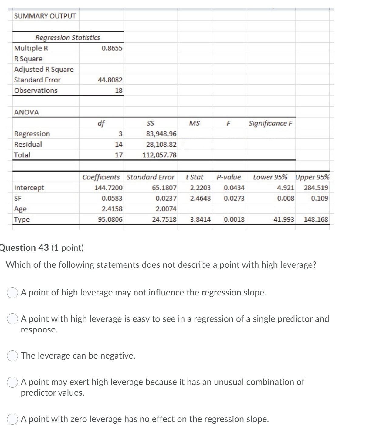
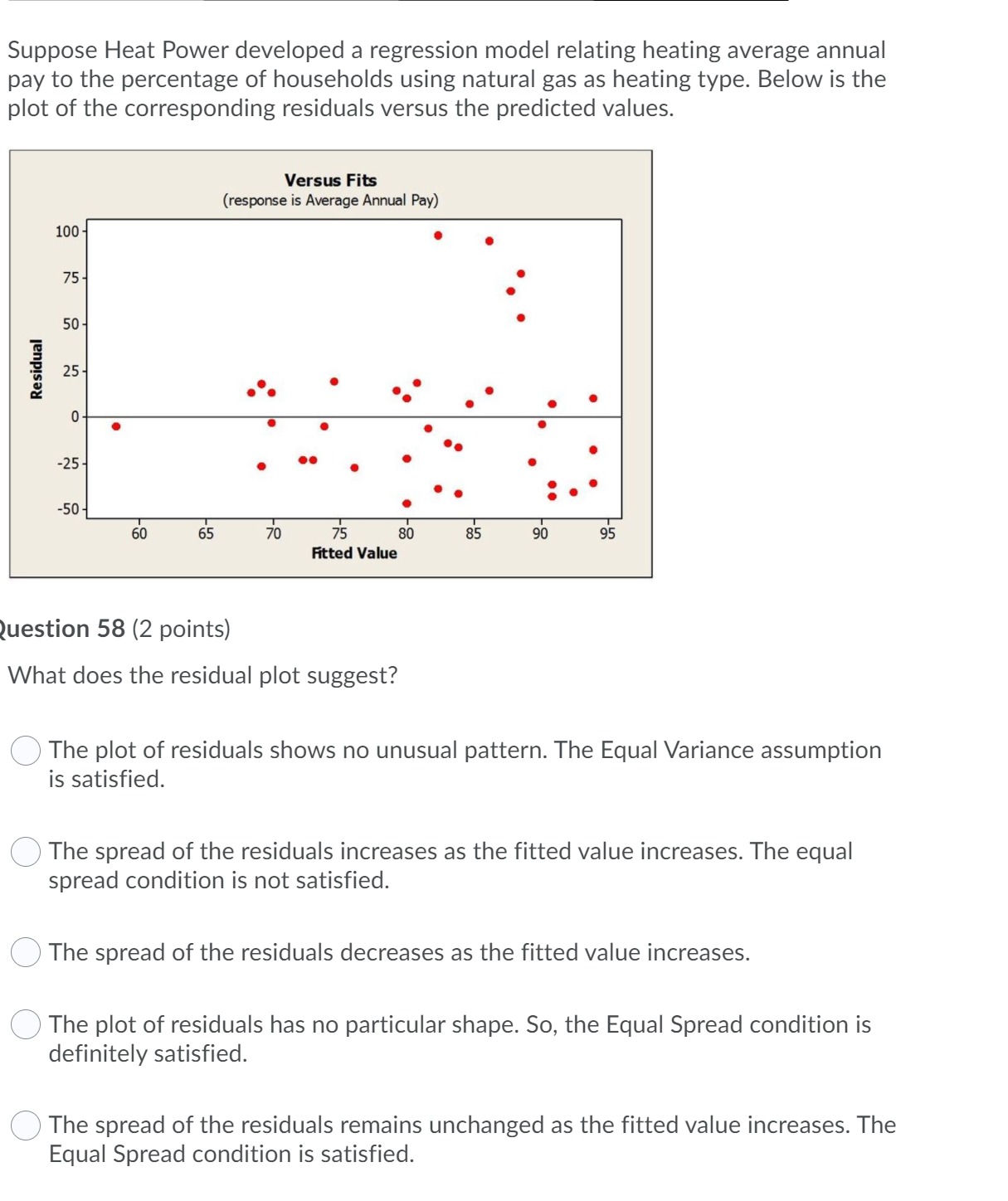
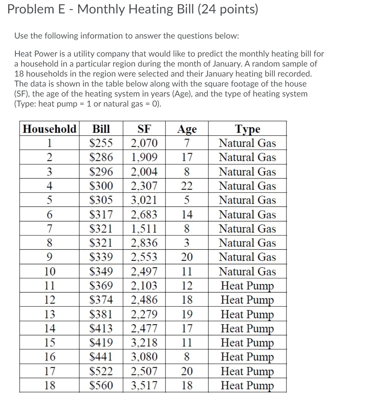
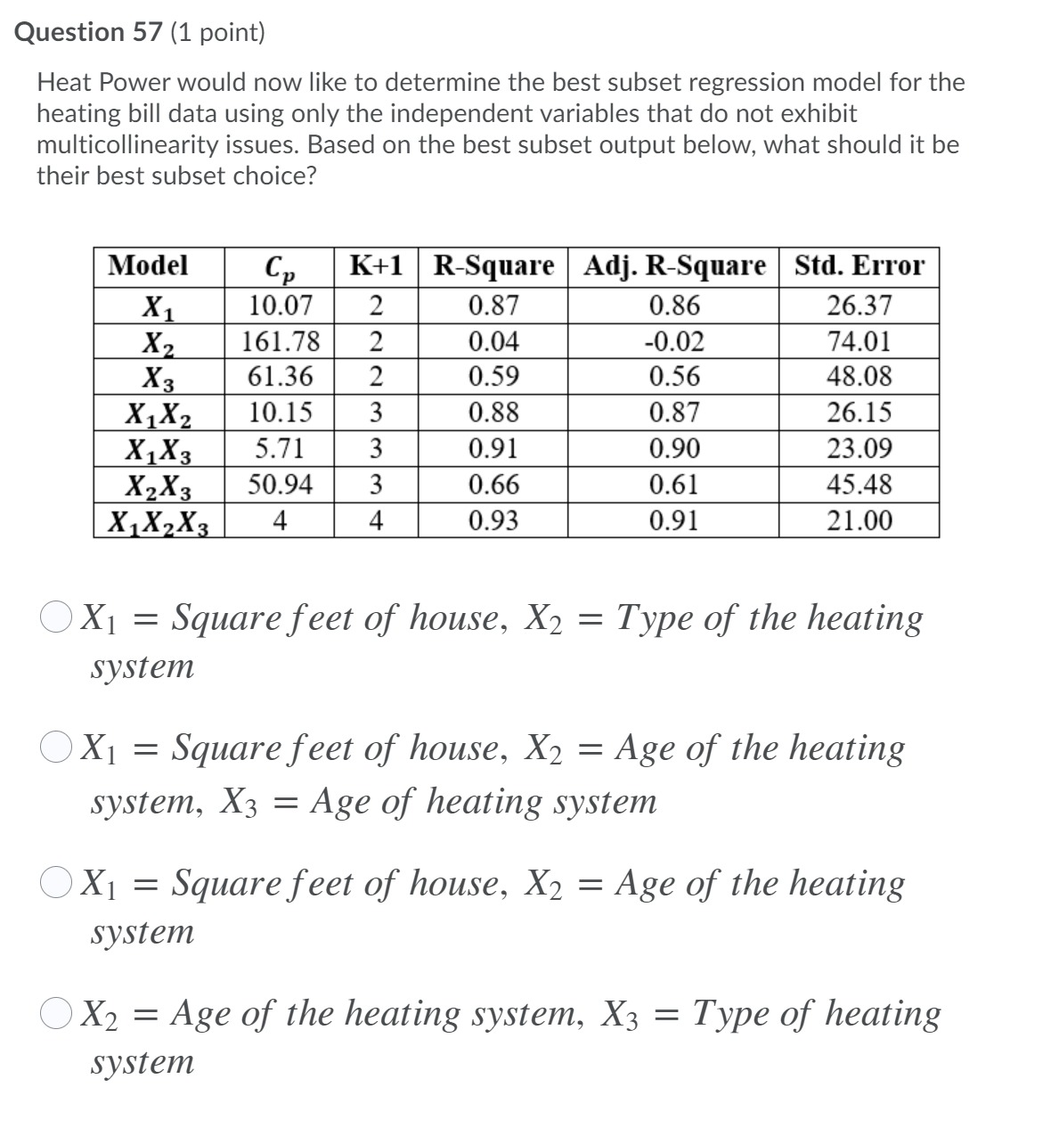
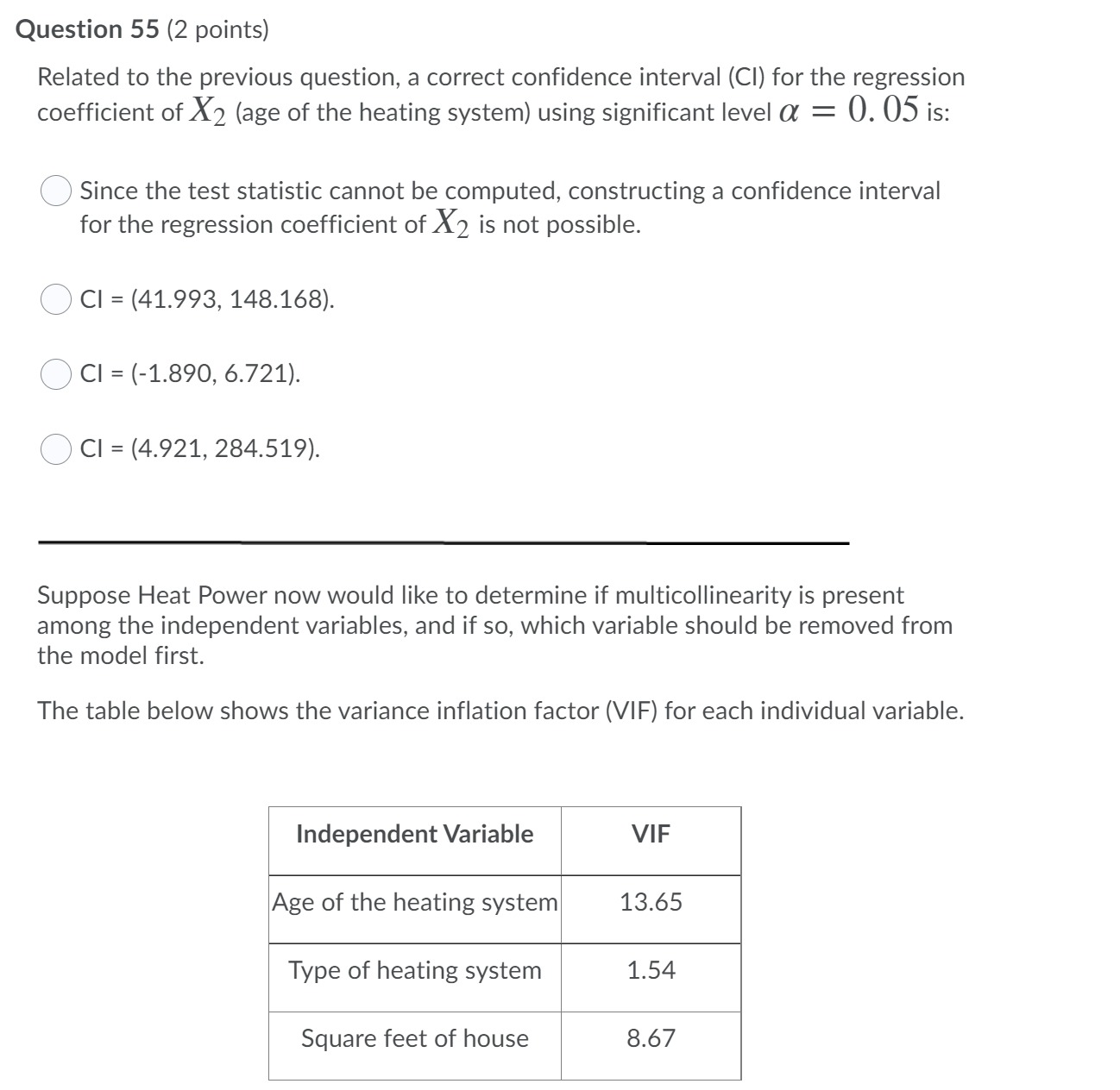
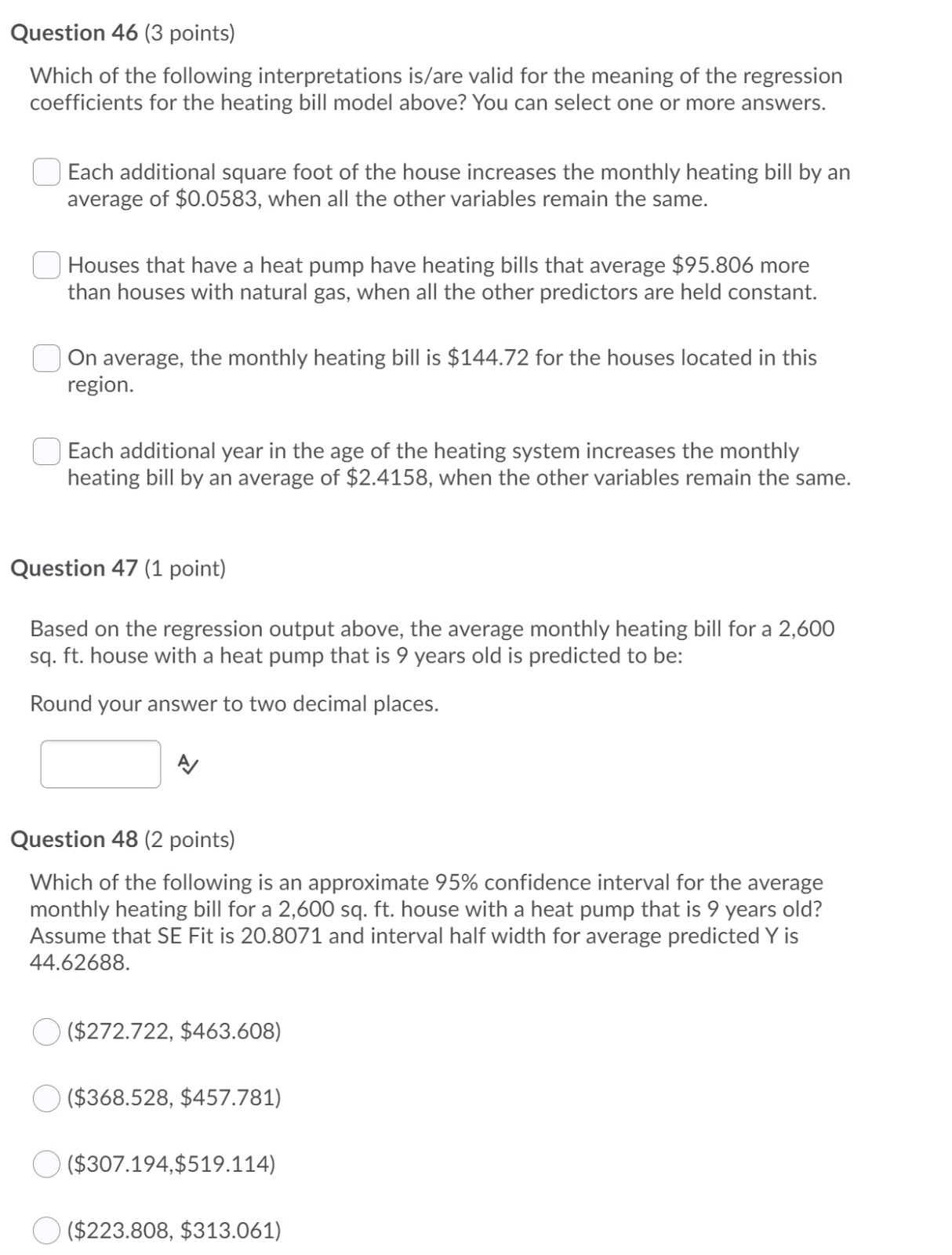
SUMMARY OUTPUT Regression Statistics Multiple R 0.8655 R Square Adjusted R Square Standard Error 44.8082 Observations 18 ANOVA df SS MS F Significance F Regression 3 83,948.96 Residual 14 28,108.82 Total 17 112,057.78 Coefficients Standard Error t Stat P-value Lower 95% Upper 95% Intercept 144.7200 65.1807 2.2203 0.0434 4.921 284.519 SF 0.0583 0.0237 2.4648 0.0273 0.008 0.109 Age 2.4158 2.0074 Type 95.0806 24.7518 3.8414 0.0018 41.993 148.168 Question 43 (1 point) Which of the following statements does not describe a point with high leverage? O A point of high leverage may not influence the regression slope. A point with high leverage is easy to see in a regression of a single predictor and response. The leverage can be negative. A point may exert high leverage because it has an unusual combination of predictor values. A point with zero leverage has no effect on the regression slope.Suppose Heat Power developed a regression model relating heating average annual pay to the percentage of households using natural gas as heating type. Below is the plot of the corresponding residuals versus the predicted values. Question 58 (2 points) What does the residual plot suggest? O The plot of residuals shows no unusual pattern. The Equal Variance assumption is satisfied. O The spread of the residuals increases as the fitted value increases. The equal spread condition is not satisfied. 0 The spread of the residuals decreases as the fitted value increases. 0 The plot of residuals has no particular shape. 50, the Equal Spread condition is definitely satisfied. 0 The spread of the residuals remains unchanged as the fitted value increases. The Equal Spread condition is satisfied. Question 4'} (2 points) Which of the following is a 95% prediction interval for the monthly heating bill for a specific house that has 2,600 square feet and a heat pump that is 9 years old? Assume that SE Fit is 20.8071 and interval half width for individual response Y is 105.9601. 0 ($307.19, $519.11) 0 ($223.808,$313.061) O ($368.528,$457.781) O The regression equation is for the average monthly heating bill, thus the monthly heating bill for a specific house cannot be computed. Question 50 (1 point) The percentage amount of the variation in a household's monthly heating bill is explained by the square footage of the house, the age of the heating system in years, and the type of heating system (heat pump or natural gas) is: Round your answer to two decimal places. l av Question 51 (2 points) Which of the following is the correct hypothesis for testing whether the regression model above is worthwhile? OH0=p1=p2 =p3 =0 H1 = at least two coefficient correlations p; 75 0 H1 2 at least l org 75 0 0H0 = 1 = 0 H1 2 l 7'5 0 OH0=151 =2 =3 =0 H1 = at least one g 7E 0 Problem E - Monthly Heating Bill (24 points) Use the following information to answer the questions below: Heat Power is a utility company that would like to predict the monthly heating bill for a household in a particular region during the month of January. A random sample of 18 households in the region were selected and their January heating bill recorded. The data is shown in the table below along with the square footage of the house (SF), the age of the heating system in years (Age), and the type of heating system (Type: heat pump = 1 or natural gas = 0). Household Bill SF Age Type $255 2,070 7 Natural Gas $286 1,909 17 Natural Gas $296 2,004 8 Natural Gas UI AWN $300 2,307 22 Natural Gas $305 3.021 5 Natural Gas $317 2,683 14 Natural Gas $321 1,511 8 Natural Gas $321 2,836 3 Natural Gas $339 2,553 20 Natural Gas 10 $349 2,497 11 Natural Gas 11 $369 2,103 12 Heat Pump 12 $374 2,486 18 Heat Pump 13 $381 2,279 19 Heat Pump 14 $413 2,477 17 Heat Pump 15 $419 3,218 11 Heat Pump 16 $441 3,080 8 Heat Pump 17 $522 2,507 20 Heat Pump 18 $560 3,517 18 Heat PumpQuestion 52 (1 point) According the summary report above, and using a significant level of a = 0. 05, we reject H0 and conclude that at least one of the population coefficients for our independent variables is not equal to zero. Question 53 (1 point} The adjusted multiple coefficient of determination for predicting a heating bill for a house in the region during the month of January is: Round you answer to two decimal places. &/ and F-statistic is . '5/ Question 54 (1 point) Which of the following is the correct test statistic associated with the significance of the regression coefficient of X2 (age of the heating system)? O F = 22203. O Calculating a test statistic is not possible for each regression coefficient since we can only test all coefficients together. O F = 1.2034. 0 F = 3.8414. Question 56 (1 point) In this regard, which of the following statements is correct? 0 Remove variable age of the heating system first ~ multicollinearity exits. C) Remove variable type of heating system first- multicollinearity does not exit. 0 Remove variable square feet of the house first multicollinearity exits. O Since multicollinearity exits for all variables, this model is not a good model for Heat Power to predict heating bills in the region. Question 59 (1 point) Considering your answer to the previous question, which of the following data transformations would be appropriate as a good start point for the response variable (average annual pay) to make it more symmetric and/or simplify its relationship with other variables? 0 Cube the data values. 0 Use a geometric transformation. 0 Square the data values. 0 Only extrapolation would help. 0 Use a logarithmic transformation. Question 44 (1 point) In order to determine whether collinearity may be an issue in the regression model, we should use: 0 Variance Inflation Factors. 0 Leverage Index. 0 Coefficient of Determination. O Cook's Distances. O Standardized Residuals. Question 45 (1 point) Based on the regression output above, which of the following regression equations would help predict the monthly heating bill for a household in the region during the month of January? Consider the following notation for the different predictor variables in the model: square footage of the house (X1), the age of the heating system(X2l, and the type of heating system(X3). ?=144.72+0.0583X1+2.4158X2+95.0806X3 O j'z'=144.72+0.0583y1+2.4158y2+95.0806y3 O ji=144.72+0.0583X1+2.4158X2+95.0806X3 Q ji=0.0583X1+2.4158X2+95.0806X3 Question 57 (1 point) Heat Power would now like to determine the best subset regression model for the heating bill data using only the independent variables that do not exhibit multicollinearity issues. Based on the best subset output below, what should it be their best subset choice? mu\" "WI m m-mxa- mun\"1- OX1 = Square feet of house, X2 2 Type of the heating system OX1 = Square feet of house, X2 2 Age of the heating system, X3 = Age of heating system OX1 = Square feet of house, X2 = Age of the heating system OX2 = Age of the heating system, X3 = Type of heating system Question 55 (2 points) Related to the previous question, a correct confidence interval (CI) for the regression coefficient of X2 (age of the heating system) using significant level a = 0. 05 is: 0 Since the test statistic cannot be computed, constructing a confidence interval for the regression coefficient of X2 is not possible. Q CI = (41.993, 148.168). Q c1 = (-1.890, 6.721). O c1 = (4.921, 284.519). Suppose Heat Power now would like to determine if multicollinearity is present among the independent variables, and if so, which variable should be removed from the model first. The table below shows the variance inflation factor (VIF) for each individual variable. Independent Variable VIF Age of the heating system 13.65 Type of heating system 1. 54 Square feet of house 8.67 Question 46 (3 points) Which of the following interpretations is/ are valid for the meaning of the regression coefficients for the heating bill model above? You can select one or more answers. C] Each additional square foot of the house increases the monthly heating bill by an average of $0.0583, when all the other variables remain the same. O Houses that have a heat pump have heating bills that average $95,806 more than houses with natural gas, when all the other predictors are held constant. [3 On average, the monthly heating bill is $144.72 for the houses located in this region. C] Each additional year in the age of the heating system increases the monthly heating bill by an average of $2.4158, when the other variables remain the same. Question 47 (1 point) Based on the regression output above, the average monthly heating bill for a 2,600 sq. ft. house with a heat pump that is 9 years old is predicted to be: Round your answer to two decimal places. Cit Question 48 (2 points) Which of the following is an approximate 95% confidence interval for the average monthly heating bill for a 2,600 sq. ft. house with a heat pump that is 9 years old? Assume that SE Fit is 20.8071 and interval half width for average predicted Y is 44.62688. 0 ($272,722, 8463.608) 0 ($368,528, $457.781) O ($307.194,$519.114) Q ($223808, $313061)