Please explain how to build this in excel

build an Excel spreadsheet to produce a chart similar to Figure 11.5 showing samples from a bivariate Student's t-distribution with four degrees of freedom where the correlation is 0.5. Next suppose that the marginal distributions of V1 and V2 are Student's t with four degrees of freedom but that a Gaussian copula with a copula correlation parameter of 0.5 is used to define the correlation between the two variables. Construct a chart showing samples from the joint distribution. Compare the two charts you have produced.

The procedure for taking a random sample from a bivariate Student's t-distribution is described on page 244. This can be used to produce Figure 11.5. For the second part of the question we samples U1 and U2 from a bivariate normal distribution where the correlation is 0.5 as described in Section 11.4. We then convert each sample into a variable with a Student's t-distribution on a 27 percentile-to-percentile basis. Suppose that U1 is in cell C1. The Excel function TINV gives a "two-tail" inverse of the t-distribution. An Excel instruction for determining V1 is therefore =IF(NORMSDIST(C1)

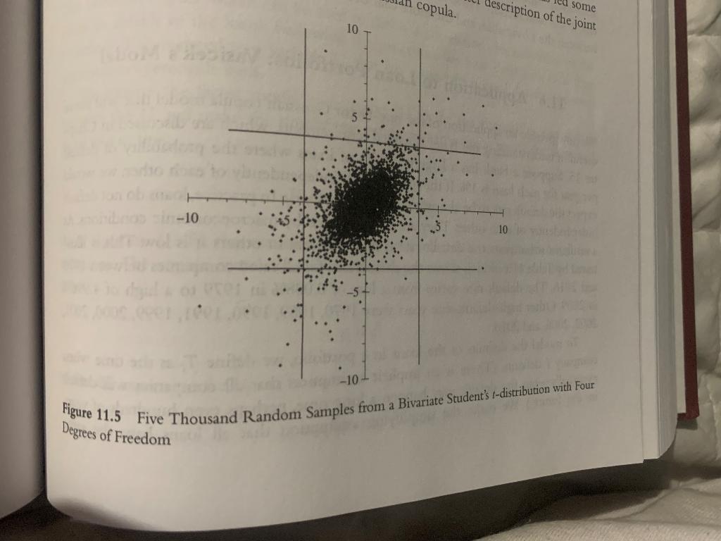
copula. description of the joint cu some 10 -10 -10 Figure 11.5 Five Thousand Random Samples from a Bivariate Student's -distribution with Four Degrees of Freedom RISK MANAGEMENT AND FINANCIAL INSTITUTIONS 244 where (.) denotes expected value and SD(.) denotes standard deviation. If there to correlation between the variables, E(VV) = E( VE(V) and p = 0.1f V, V.be nerator and the denominator in the expression for p equal the variance of Vih we would expect, p = 1 in this case. The covariance between V, and V, is defined as cov(V1, V2) = E(V, V3) - E(V)E(V2) so that the correlation can be written , bolo cov(V1, V2) SD(V1) SD (V2) P Although it is easier to develop intuition about the meaning of a correlation in covariance, it is covariances that will prove to be the fundamental variables of our analys An analogy here is that variance rates were the fundamental variables for the EWMA and GARCH models in Chapter 10, even though it is easier to develop intuition abou volatilities. 11.1.1 Correlation vs. Dependence Two variables are defined as statistically independent if knowledge about one of them does not affect the probability distribution for the other. Formally, V, and are inde pendent it: Figu S(V2V = x) = f(V) expe consi cient Vi au enco of V incre A stand V, an devia for all x where f(a) denotes the probability density function and is the symbol denoting "conditional on. If the coefficient of correlation between two variables is zero, does this mean die there is no dependence between the variables? The answer is no. We can illustrate than with a simple example. Suppose that there are three equally likely values for Vio and +1.18 V, = -1 or vi = +1, then V = +1. If V, = 0, then V, = 0. In this case, there is clearly a dependence between V, and V,. If we observe the value of V, we know the value of V2. Also, a knowledge of the value of V will cause us to change our probably distribution for V1. However, because EV V) = 0 and E(V) = 0, it is easy to see the the coefficient of correlation between V, and V2 is zero. particular type of dependence between two variables. This is linear dependence. There are This example emphasizes the point that the coefficient of correlation measures many other ways in which two variables can be related. We can characterize the nature shown in Figure 11.1. Figure 11.1(a) shows linear dependence where the expected value the dependence between V, and V, by plotting E(V2) against V. Three examples of V, depends linearly on V. Figure 11.1(b) shows a V-shaped relationship between Chap can be used of av WO copula. description of the joint cu some 10 -10 -10 Figure 11.5 Five Thousand Random Samples from a Bivariate Student's -distribution with Four Degrees of Freedom RISK MANAGEMENT AND FINANCIAL INSTITUTIONS 244 where (.) denotes expected value and SD(.) denotes standard deviation. If there to correlation between the variables, E(VV) = E( VE(V) and p = 0.1f V, V.be nerator and the denominator in the expression for p equal the variance of Vih we would expect, p = 1 in this case. The covariance between V, and V, is defined as cov(V1, V2) = E(V, V3) - E(V)E(V2) so that the correlation can be written , bolo cov(V1, V2) SD(V1) SD (V2) P Although it is easier to develop intuition about the meaning of a correlation in covariance, it is covariances that will prove to be the fundamental variables of our analys An analogy here is that variance rates were the fundamental variables for the EWMA and GARCH models in Chapter 10, even though it is easier to develop intuition abou volatilities. 11.1.1 Correlation vs. Dependence Two variables are defined as statistically independent if knowledge about one of them does not affect the probability distribution for the other. Formally, V, and are inde pendent it: Figu S(V2V = x) = f(V) expe consi cient Vi au enco of V incre A stand V, an devia for all x where f(a) denotes the probability density function and is the symbol denoting "conditional on. If the coefficient of correlation between two variables is zero, does this mean die there is no dependence between the variables? The answer is no. We can illustrate than with a simple example. Suppose that there are three equally likely values for Vio and +1.18 V, = -1 or vi = +1, then V = +1. If V, = 0, then V, = 0. In this case, there is clearly a dependence between V, and V,. If we observe the value of V, we know the value of V2. Also, a knowledge of the value of V will cause us to change our probably distribution for V1. However, because EV V) = 0 and E(V) = 0, it is easy to see the the coefficient of correlation between V, and V2 is zero. particular type of dependence between two variables. This is linear dependence. There are This example emphasizes the point that the coefficient of correlation measures many other ways in which two variables can be related. We can characterize the nature shown in Figure 11.1. Figure 11.1(a) shows linear dependence where the expected value the dependence between V, and V, by plotting E(V2) against V. Three examples of V, depends linearly on V. Figure 11.1(b) shows a V-shaped relationship between Chap can be used of av WO