please help in providing a worksheet . thank you so much

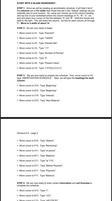
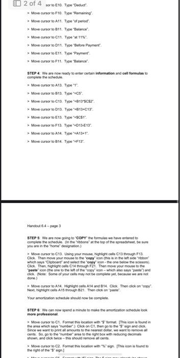
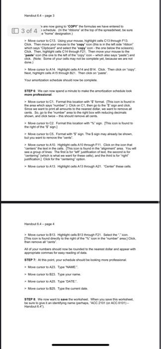
START WITH A BLANK WORKSHEET. STEP 1: Since we wil be creating an amortization schedule, it wil help if al of the columns are a lifte wider than those that are in the "defaur" seltings fas you oniginally see on your screen). So, using your mouse, 90 to the column heading (the top line of your worksheet where the column headings of " A ", " B ", " C ", etc. are) and place your cursor on the line between " A " and " B ". Hold the mouse and slide to the right. This will widen the column. Do this for each column (A through F). Move to a width of about 14. STEP 2: We are now ready to begin. > Move cursor to A1. Type Paymenr. > Move cursor to C1. Type "120000". Move curscor to A2. Type "interest rate" > Move cursor to C2. Type *11". > Move cursor to A3. Type "Number of Periads". > Move cursor to C3. Type "9". > Move cursor to AS. Type "Present Value". > Move eursor to C5. Type "-pV(C2.C3.C1)". STEP 3: We are now ready to prepace the schedule. First move cursce to C8, type "AMORTIZATION SCHEDULE", Noxt, we will type the headings for each column. > Move cursor to A10. Type "Beginning", > Move cursor to B10. Type "Beginning". > Move cursor to C10. Type "Interest". > Move cursor to D10. Type "New Bulance". Handout 6.4 page 2 > Move cursor to E10. Type "Deducr: > Move cursor to F10. Type "Remaining". > Move cursor to A11, Type "of period". > Move cursor to B11. Type "Balance". > Move cursor to C11. Type "at 11:" > Move cursor to D11. Type "Belore Payment". > Move cursor to E11. Type 'Paymenf > Move cursor to F11. Type "Balance". STEP 4: We are now ready to enter certain information and cell formulas to complete the schedule. > Move cursor to A13. Type "1". > Move cursor to B13. Type " =C5 " 2 of 4 wer to Eso. Type Deduer. > Move cussor to F10. Type "Remaining". ? Move curvor to A11. Type "of penod". > Move cursor to B11. Type "Bulince". > Move cursor to C11. Type "at 11N2. > Move cursor to D11. Type "Betome Payment. > Mowe cuncr to E11. Type "Payment". > Move cursor to F11. Type "Baince". STEP 4: We are now teady to enter certain information and cell formulas ito complete the schedule. > Move cursor to A13. Type 4: > Move cursor to B13. Type " =C5. > Move aunor to C13. Type "ra1s'sCse" > Move cuncr to D13. Type "ug13+C13". > Move cursor to E13. Type "nsC51". > Move curtor to F13. Type "=D13-E13: > Move cursor to A14, Type " =0 A13+ 12, > Move cursor to B14. Type "nF13" Handeut 6.4 page 3 STEP 5. We are now going to "COPY the formulas wee have eniered to complete the schedule. fin the "rbbons' at the top of the spreactaheot. be sure you are in the Theme" designation. > Move cursor to C13. Using your mouse, hightight cells C13 through F13. Click. Then move your mouse to the "copy' icon (this is in the lot side "ribbon' which says "Clipboand" and select the "copy" ioce - the one below pe scissors:. Click. Then, highlight cels C14 through F21. Then move your mouse to the "paste" icon (the one to the left dof the "copy" icon - which also sars "paste") and click. (Note: Some of your colls may not be complete yet, becante we are not doret.) > Move cursor to A14. Highlight cells A14 and B14. Click. Then click on "copy". Your amortiusion schedule should now be complete. STEP 6: We can now spend a minule to make the amortization schedule lock more professional the area which surs "fumber', ) Click on C1, then go to the " $ " sign and click. Since we want to print all amovints to the nearest dolac, we wart to remove ail cents. So, go to the "number' area to the right bor wth reducing decimals shown. and click falce - this should remove all cents. the fight of the -5 sign] 3 of 4 trare now gaing to tcopr the formulat we have entered the e "home" dosignation.) ? Move cursor to C\$3. Uaing your mouse, Nighliont eels C13 through F13 which says "Clpboend" and select the "eopy' koon - the one below the sciesom! Click. Then, highlight cells C14 trough F2! Theo move your mouse to the done ) > Move curwor to A.M. Highlight cels A14 and B14. Click. Theo dick on "bepy. Neet, tighlight cells A15 though B21. Then olok on "paute" Your amortzison schoble should now be esenplene. 5TEP 6. We can now ssend a minste to make the amontzation schedile iock. more professional. the ave which says "number' is Click on C1, flen go to the 's sign and click. Since ep wart to print all amounts to the noarest dolar, we nank to remove all eents. So. go to the 'number' area is the fighe box with seducing deciman thown, and dick teice - this shouid fenove at cents. the right of the " t " sign. > Move curser to C5. Format with " $ "sign. The $ sigo mary aboady be shown. bul you wart bo remove the "chents"? > Mous courso to A to. Highlight cells A10 fupugh F11. Click on the ioon that "centering" (which is what wo waret for these cells), and the thind in for "righer justication. Click, for the "eantaring" option. > Move cursor is A13. Highlight cels A.13 through A21. Carter these dabs. Mandout 6.4-poge 4 7 Move carser to B13. Highight cels B13 through F21. Silect the *; kan. then nempove all "conts" Al of your numbers shoud now be rounded to the nearest dolor and appear wen appropriate cimmas tor eatry natading of data. STEP 7: At thes point, your schedde should be looking more prolessiona: > Move curnor is A23. Type "NAME" > Move carsor b B23. Type your name. > Move curvor to N2S. Type 'DaTE" > Move cursor to B25. Type the currest dabe. STEP 1. We now want to save the worksheet. When you save the =orksheet. be sure to give it an identiping name (perthes, "ACC 2tot (or ACC Eto1) Handoun 6.4 ? 7 . START WITH A BLANK WORKSHEET. STEP 1: Since we wil be creating an amortization schedule, it wil help if al of the columns are a lifte wider than those that are in the "defaur" seltings fas you oniginally see on your screen). So, using your mouse, 90 to the column heading (the top line of your worksheet where the column headings of " A ", " B ", " C ", etc. are) and place your cursor on the line between " A " and " B ". Hold the mouse and slide to the right. This will widen the column. Do this for each column (A through F). Move to a width of about 14. STEP 2: We are now ready to begin. > Move cursor to A1. Type Paymenr. > Move cursor to C1. Type "120000". Move curscor to A2. Type "interest rate" > Move cursor to C2. Type *11". > Move cursor to A3. Type "Number of Periads". > Move cursor to C3. Type "9". > Move cursor to AS. Type "Present Value". > Move eursor to C5. Type "-pV(C2.C3.C1)". STEP 3: We are now ready to prepace the schedule. First move cursce to C8, type "AMORTIZATION SCHEDULE", Noxt, we will type the headings for each column. > Move cursor to A10. Type "Beginning", > Move cursor to B10. Type "Beginning". > Move cursor to C10. Type "Interest". > Move cursor to D10. Type "New Bulance". Handout 6.4 page 2 > Move cursor to E10. Type "Deducr: > Move cursor to F10. Type "Remaining". > Move cursor to A11, Type "of period". > Move cursor to B11. Type "Balance". > Move cursor to C11. Type "at 11:" > Move cursor to D11. Type "Belore Payment". > Move cursor to E11. Type 'Paymenf > Move cursor to F11. Type "Balance". STEP 4: We are now ready to enter certain information and cell formulas to complete the schedule. > Move cursor to A13. Type "1". > Move cursor to B13. Type " =C5 " 2 of 4 wer to Eso. Type Deduer. > Move cussor to F10. Type "Remaining". ? Move curvor to A11. Type "of penod". > Move cursor to B11. Type "Bulince". > Move cursor to C11. Type "at 11N2. > Move cursor to D11. Type "Betome Payment. > Mowe cuncr to E11. Type "Payment". > Move cursor to F11. Type "Baince". STEP 4: We are now teady to enter certain information and cell formulas ito complete the schedule. > Move cursor to A13. Type 4: > Move cursor to B13. Type " =C5. > Move aunor to C13. Type "ra1s'sCse" > Move cuncr to D13. Type "ug13+C13". > Move cursor to E13. Type "nsC51". > Move curtor to F13. Type "=D13-E13: > Move cursor to A14, Type " =0 A13+ 12, > Move cursor to B14. Type "nF13" Handeut 6.4 page 3 STEP 5. We are now going to "COPY the formulas wee have eniered to complete the schedule. fin the "rbbons' at the top of the spreactaheot. be sure you are in the Theme" designation. > Move cursor to C13. Using your mouse, hightight cells C13 through F13. Click. Then move your mouse to the "copy' icon (this is in the lot side "ribbon' which says "Clipboand" and select the "copy" ioce - the one below pe scissors:. Click. Then, highlight cels C14 through F21. Then move your mouse to the "paste" icon (the one to the left dof the "copy" icon - which also sars "paste") and click. (Note: Some of your colls may not be complete yet, becante we are not doret.) > Move cursor to A14. Highlight cells A14 and B14. Click. Then click on "copy". Your amortiusion schedule should now be complete. STEP 6: We can now spend a minule to make the amortization schedule lock more professional the area which surs "fumber', ) Click on C1, then go to the " $ " sign and click. Since we want to print all amovints to the nearest dolac, we wart to remove ail cents. So, go to the "number' area to the right bor wth reducing decimals shown. and click falce - this should remove all cents. the fight of the -5 sign] 3 of 4 trare now gaing to tcopr the formulat we have entered the e "home" dosignation.) ? Move cursor to C\$3. Uaing your mouse, Nighliont eels C13 through F13 which says "Clpboend" and select the "eopy' koon - the one below the sciesom! Click. Then, highlight cells C14 trough F2! Theo move your mouse to the done ) > Move curwor to A.M. Highlight cels A14 and B14. Click. Theo dick on "bepy. Neet, tighlight cells A15 though B21. Then olok on "paute" Your amortzison schoble should now be esenplene. 5TEP 6. We can now ssend a minste to make the amontzation schedile iock. more professional. the ave which says "number' is Click on C1, flen go to the 's sign and click. Since ep wart to print all amounts to the noarest dolar, we nank to remove all eents. So. go to the 'number' area is the fighe box with seducing deciman thown, and dick teice - this shouid fenove at cents. the right of the " t " sign. > Move curser to C5. Format with " $ "sign. The $ sigo mary aboady be shown. bul you wart bo remove the "chents"? > Mous courso to A to. Highlight cells A10 fupugh F11. Click on the ioon that "centering" (which is what wo waret for these cells), and the thind in for "righer justication. Click, for the "eantaring" option. > Move cursor is A13. Highlight cels A.13 through A21. Carter these dabs. Mandout 6.4-poge 4 7 Move carser to B13. Highight cels B13 through F21. Silect the *; kan. then nempove all "conts" Al of your numbers shoud now be rounded to the nearest dolor and appear wen appropriate cimmas tor eatry natading of data. STEP 7: At thes point, your schedde should be looking more prolessiona: > Move curnor is A23. Type "NAME" > Move carsor b B23. Type your name. > Move curvor to N2S. Type 'DaTE" > Move cursor to B25. Type the currest dabe. STEP 1. We now want to save the worksheet. When you save the =orksheet. be sure to give it an identiping name (perthes, "ACC 2tot (or ACC Eto1) Handoun 6.4 ? 7