Please help with this assignment. Part two : Compute Loss def grad(beta, b, xTr, yTr, xTe, yTe, C, kerneltype, kpar=1):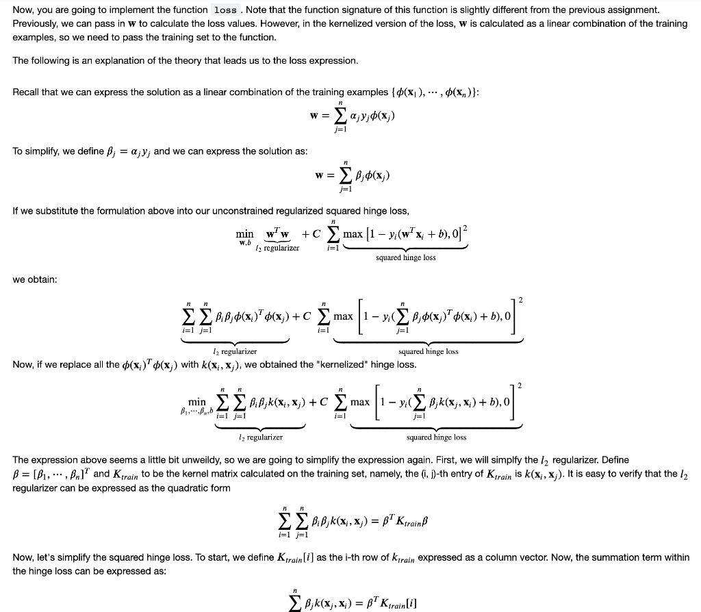

Test Cases for part 2 :

# These tests test whether your loss() is implemented correctly

xTr_test, yTr_test = generate_data() n, d = xTr_test.shape

# Check whether your loss() returns a scalar def loss_test1(): beta = np.zeros(n) b = np.zeros(1) loss_val = loss(beta, b, xTr_test, yTr_test, xTr_test, yTr_test, 10, 'rbf') return np.isscalar(loss_val)

# Check whether your loss() returns a nonnegative scalar def loss_test2(): beta = np.random.rand(n) b = np.random.rand(1) loss_val = loss(beta, b, xTr_test, yTr_test, xTr_test, yTr_test, 10, 'rbf') return loss_val >= 0

# Check whether you implement l2-regularizer correctly def loss_test3(): beta = np.random.rand(n) b = np.random.rand(1) loss_val = loss(beta, b, xTr_test, yTr_test, xTr_test, yTr_test, 0, 'rbf') loss_val_grader = loss_grader(beta, b, xTr_test, yTr_test, xTr_test, yTr_test, 0, 'rbf') return (np.linalg.norm(loss_val - loss_val_grader)

loss_test3()

# Check whether you implement square hinge loss correctly def loss_test4(): beta = np.zeros(n) b = np.random.rand(1) loss_val = loss(beta, b, xTr_test, yTr_test, xTr_test, yTr_test, 10, 'rbf') loss_val_grader = loss_grader(beta, b, xTr_test, yTr_test, xTr_test, yTr_test, 10, 'rbf') return (np.linalg.norm(loss_val - loss_val_grader)

# Check whether you implement square hinge loss correctly def loss_test5(): beta = np.zeros(n) b = np.random.rand(1) loss_val = loss(beta, b, xTr_test, yTr_test, xTr_test, yTr_test, 10, 'rbf') loss_val_grader = loss_grader(beta, b, xTr_test, yTr_test, xTr_test, yTr_test, 10, 'rbf') return (np.linalg.norm(loss_val - loss_val_grader)

# Check whether you implement loss correctly def loss_test6(): beta = np.zeros(n) b = np.random.rand(1) loss_val = loss(beta, b, xTr_test, yTr_test, xTr_test, yTr_test, 100, 'rbf') loss_val_grader = loss_grader(beta, b, xTr_test, yTr_test, xTr_test, yTr_test, 100, 'rbf') return (np.linalg.norm(loss_val - loss_val_grader)

runtest(loss_test1,'loss_test1') runtest(loss_test2,'loss_test2') runtest(loss_test3,'loss_test3') runtest(loss_test4,'loss_test4') runtest(loss_test5,'loss_test5') runtest(loss_test6,'loss_test6')

Part Three : Compute Gradient def grad(beta, b, xTr, yTr, xTe, yTe, C, kerneltype, kpar=1):

Test cases for part 4:

# These tests test whether your grad() is implemented correctly

xTr_test, yTr_test = generate_data() n, d = xTr_test.shape

# Checks whether grad returns a tuple def grad_test1(): beta = np.random.rand(n) b = np.random.rand(1) out = grad(beta, b, xTr_test, yTr_test, xTr_test, yTr_test, 10, 'rbf') return len(out) == 2

# Checks the dimension of gradients def grad_test2(): beta = np.random.rand(n) b = np.random.rand(1) beta_grad, bgrad = grad(beta, b, xTr_test, yTr_test, xTr_test, yTr_test, 10, 'rbf') return len(beta_grad) == n and np.isscalar(bgrad)

# Checks the gradient of the l2 regularizer def grad_test3(): beta = np.random.rand(n) b = np.random.rand(1) beta_grad, bgrad = grad(beta, b, xTr_test, yTr_test, xTr_test, yTr_test, 0, 'rbf') beta_grad_grader, bgrad_grader = grad_grader(beta, b, xTr_test, yTr_test, xTr_test, yTr_test, 0, 'rbf') return (np.linalg.norm(beta_grad - beta_grad_grader)

# Checks the gradient of the square hinge loss def grad_test4(): beta = np.zeros(n) b = np.random.rand(1) beta_grad, bgrad = grad(beta, b, xTr_test, yTr_test, xTr_test, yTr_test, 1, 'rbf') beta_grad_grader, bgrad_grader = grad_grader(beta, b, xTr_test, yTr_test, xTr_test, yTr_test, 1, 'rbf') return (np.linalg.norm(beta_grad - beta_grad_grader)

# Checks the gradient of the loss def grad_test5(): beta = np.random.rand(n) b = np.random.rand(1) beta_grad, bgrad = grad(beta, b, xTr_test, yTr_test, xTr_test, yTr_test, 10, 'rbf') beta_grad_grader, bgrad_grader = grad_grader(beta, b, xTr_test, yTr_test, xTr_test, yTr_test, 10, 'rbf') return (np.linalg.norm(beta_grad - beta_grad_grader)

runtest(grad_test1, 'grad_test1') runtest(grad_test2, 'grad_test2') runtest(grad_test3, 'grad_test3') runtest(grad_test4, 'grad_test4') runtest(grad_test5, 'grad_test5')

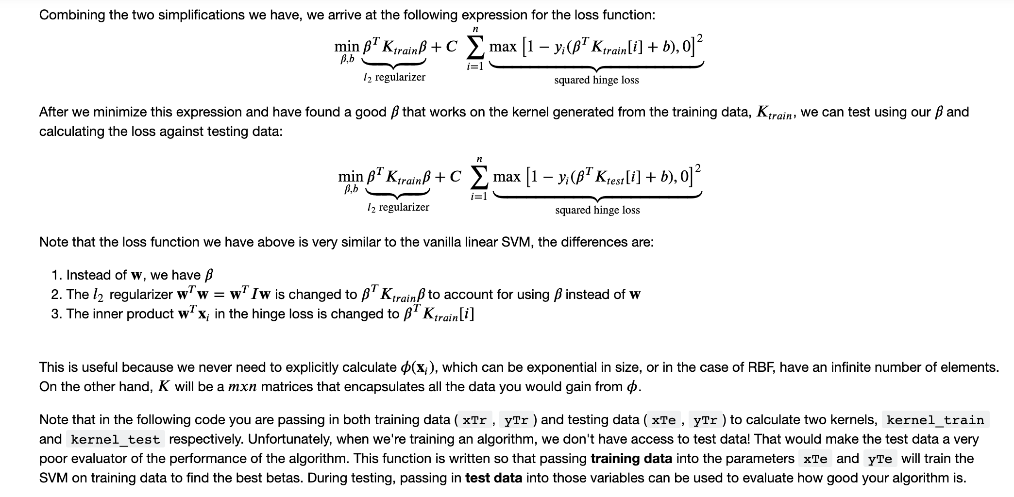
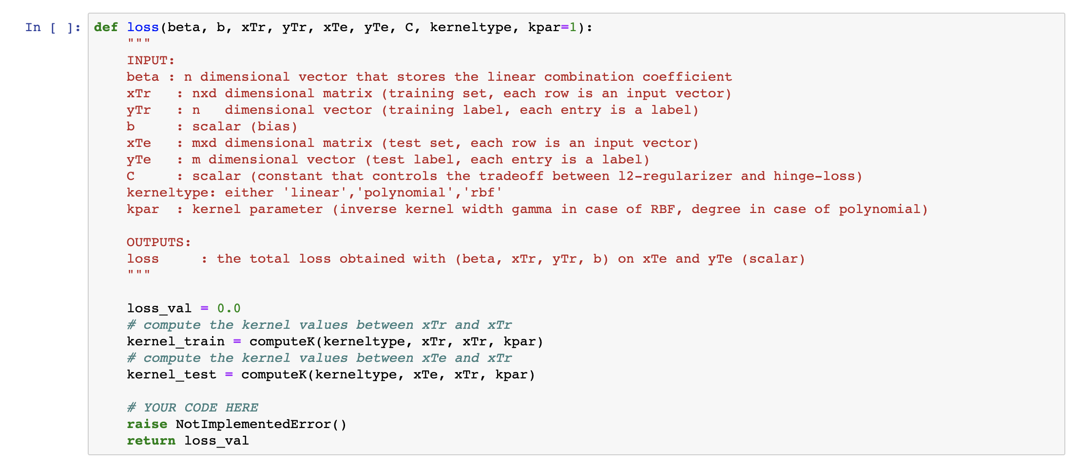
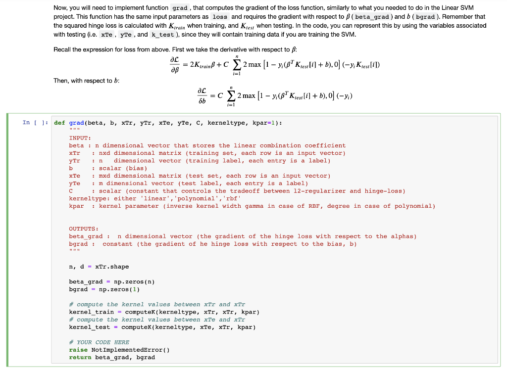
Now, you are going to implement the function loss . Note that the function signature of this function is slightly different from the previous assignment. Previously, we can pass in w to calculate the loss values. However, in the kernelized version of the loss, w is calculated as a linear combination of the training examples, so we need to pass the training set to the function. The following is an explanation of the theory that leads us to the loss expression. Recall that we can express the solution as a linear combination of the training examples {(xi), ..., 4(x)}: 24;y;"(x;) J=1 To simplify, we define B; = a;y; and we can express the solution as: W= Bj(x)) j=1 If we substitute the formulation above into our unconstrained regularized squared hinge loss, min w w +C max (1 y/(w"x + w.b 12 regularizer i=1 squared hinge loss +b), 0] we obtain: n P.B;$(x)?d[x;) +C 3 max [13 now,*box) +0,0) i=1 j=1 i=1 12 regularizer squared hinge loss Now, if we replace all the p(x)+(x;) with k(x, X;), we obtained the "kernelized" hinge loss. PI PL minEEB:B;kx,x) + C max 1 - vic B;k(x;, X;) + b), 0 i=1 j=1 i= 12 regularizer squared hinge loss The expression above seems a little bit unweildy, so we are going to simplify the expression again. First, we will simplfy the l2 regularizer. Define B = [B1,.,Br]" and Kyrain to be the kernel matrix calculated on the training set, namely, the (i, j)-th entry of Ktrain is k(x,x;). It is easy to verify that the l2 regularizer can be expressed as the quadratic form 23 B.B,k(x), x)) = b^ Kiraim i=1 =1 Now, let's simplify the squared hinge loss. To start, we define Kirain[i] as the i-th row of Ktrain expressed as a column vector. Now, the summation term within the hinge loss can be expressed as: BK B;k(x,x) = BT Kirain [i] n Combining the two simplifications we have, we arrive at the following expression for the loss function: y;[i+ B,b i=1 12 regularizer squared hinge loss After we minimize this expression and have found a good that works on the kernel generated from the training data, Ktrain, we can test using our and calculating the loss against testing data: n min B7 KtrainB + C E max [1 yi(b? Ktest [i] + b), 0]? Bb i=1 12 regularizer squared hinge loss Note that the loss function we have above is very similar to the vanilla linear SVM, the differences are: 1. Instead of w, we have B 2. The la regularizer w w = w Iw is changed to Ktrain to account for using instead of w 3. The inner product w x; in the hinge loss is changed to Ktrain[i] This is useful because we never need to explicitly calculate $(x;), which can be exponential in size, or in the case of RBF, have an infinite number of elements. On the other hand, K will be a mxn matrices that encapsulates all the data you would gain from 0. Note that in the following code you are passing in both training data ( xTr , yTr ) and testing data ( xTe , yTr ) to calculate two kernels, kernel_train and kernel_test respectively. Unfortunately, when we're training an algorithm, we don't have access to test data! That would make the test data a very poor evaluator of the performance of the algorithm. This function is written so that passing training data into the parameters xTe and yte will train the SVM on training data to find the best betas. During testing, passing in test data into those variables can be used to evaluate how good your algorithm is. In [ ]: def loss (beta, b, xTr, ytr, xTe, yte, C, kerneltype, kpar=1): . n : INPUT: beta : n dimensional vector that stores the linear combination coefficient xTr : nxd dimensional matrix (training set, each row is an input vector) yTr dimensional vector (training label, each entry is a label) b scalar (bias) xTe : mxd dimensional matrix (test set, each row is an input vector) : m dimensional vector (test label, each entry is a label) : scalar (constant that controls the tradeoff between 12-regularizer and hinge-loss) kerneltype: either 'linear', 'polynomial', 'rbf' kpar : kernel parameter (inverse kernel width gamma in case of RBF, degree in case of polynomial) OUTPUTS: loss the total loss obtained with (beta, xTr, ytr, b) on xTe and yte (scalar) loss_val = 0.0 # compute the kernel values between xtr and Tr kernel_train computek(kerneltype, xTr, xTr, kpar) # compute the kernel values between xTe and xtr kernel_test = computek(kerneltype, xTe, Tr, kpar) # YOUR CODE HERE raise No nplementedError() return loss_val Now, you will need to implement function grad, that computes the gradient of the loss function, similarly to what you needed to do in the Linear SVM project. This function has the same input parameters as loss and requires the gradient with respect to (beta_grad) and b (bgrad ). Remember that the squared hinge loss is calculated with Ktrain when training, and Kjes when testing. In the code, you can represent this by using the variables associated with testing (i.e. xte, yTe , and k_test), since they will contain training data if you are training the SVM. i=1 Recall the expression for loss from above. First we take the derivative with respect to : ac = 2Ktrain +C 2 max (1 y;(Ktes: [i] + b), 0] (-y;Ktesi [i]) Then, with respect to b: ac =C 2 max (1 y;(87Kiest [i] + b), O] (-y;) 8b i=1 In [ ]: def grad(beta, b, xTr, ytr, xTe, yte, c, kerneltype, kpar=1): INPUT: b beta : n dimensional vector that stores the linear combination coefficient xTr : nxd dimensional matrix (training set, each row is an input vector) yTr dimensional vector (training label, each entry is a label) : scalar (bias) xTe : mxd dimensional matrix (test set, each row is an input vector) : m dimensional vector (test label, each entry is a label) : scalar (constant that controls the tradeoff between 12-regularizer and hinge-loss) kerneltype: either 'linear', 'polynomial', 'rbf' kpar : kernel parameter (inverse kernel width gamma in case of RBF, degree in case of polynomial) OUT beta grad: n dimensional vector (the gradient of the hinge loss with respect to the alphas) bgrad: constant (the gradient of he hinge loss with respect to the bias, b) HI n, d = xTr.shape beta grad = np.zeros(n) bgrad = np.zeros(1) # compute the kernel values between xtr and xtr kernel_train = computek (kerneltype, xtr, xtr, kpar) # compute the kernel values between xTe and xtr kernel_test - computek(kerneltype, xTe, xtr, kpar) # YOUR CODE HERE raise Not ImplementedError() return beta_grad, bgrad Now, you are going to implement the function loss . Note that the function signature of this function is slightly different from the previous assignment. Previously, we can pass in w to calculate the loss values. However, in the kernelized version of the loss, w is calculated as a linear combination of the training examples, so we need to pass the training set to the function. The following is an explanation of the theory that leads us to the loss expression. Recall that we can express the solution as a linear combination of the training examples {(xi), ..., 4(x)}: 24;y;"(x;) J=1 To simplify, we define B; = a;y; and we can express the solution as: W= Bj(x)) j=1 If we substitute the formulation above into our unconstrained regularized squared hinge loss, min w w +C max (1 y/(w"x + w.b 12 regularizer i=1 squared hinge loss +b), 0] we obtain: n P.B;$(x)?d[x;) +C 3 max [13 now,*box) +0,0) i=1 j=1 i=1 12 regularizer squared hinge loss Now, if we replace all the p(x)+(x;) with k(x, X;), we obtained the "kernelized" hinge loss. PI PL minEEB:B;kx,x) + C max 1 - vic B;k(x;, X;) + b), 0 i=1 j=1 i= 12 regularizer squared hinge loss The expression above seems a little bit unweildy, so we are going to simplify the expression again. First, we will simplfy the l2 regularizer. Define B = [B1,.,Br]" and Kyrain to be the kernel matrix calculated on the training set, namely, the (i, j)-th entry of Ktrain is k(x,x;). It is easy to verify that the l2 regularizer can be expressed as the quadratic form 23 B.B,k(x), x)) = b^ Kiraim i=1 =1 Now, let's simplify the squared hinge loss. To start, we define Kirain[i] as the i-th row of Ktrain expressed as a column vector. Now, the summation term within the hinge loss can be expressed as: BK B;k(x,x) = BT Kirain [i] n Combining the two simplifications we have, we arrive at the following expression for the loss function: y;[i+ B,b i=1 12 regularizer squared hinge loss After we minimize this expression and have found a good that works on the kernel generated from the training data, Ktrain, we can test using our and calculating the loss against testing data: n min B7 KtrainB + C E max [1 yi(b? Ktest [i] + b), 0]? Bb i=1 12 regularizer squared hinge loss Note that the loss function we have above is very similar to the vanilla linear SVM, the differences are: 1. Instead of w, we have B 2. The la regularizer w w = w Iw is changed to Ktrain to account for using instead of w 3. The inner product w x; in the hinge loss is changed to Ktrain[i] This is useful because we never need to explicitly calculate $(x;), which can be exponential in size, or in the case of RBF, have an infinite number of elements. On the other hand, K will be a mxn matrices that encapsulates all the data you would gain from 0. Note that in the following code you are passing in both training data ( xTr , yTr ) and testing data ( xTe , yTr ) to calculate two kernels, kernel_train and kernel_test respectively. Unfortunately, when we're training an algorithm, we don't have access to test data! That would make the test data a very poor evaluator of the performance of the algorithm. This function is written so that passing training data into the parameters xTe and yte will train the SVM on training data to find the best betas. During testing, passing in test data into those variables can be used to evaluate how good your algorithm is. In [ ]: def loss (beta, b, xTr, ytr, xTe, yte, C, kerneltype, kpar=1): . n : INPUT: beta : n dimensional vector that stores the linear combination coefficient xTr : nxd dimensional matrix (training set, each row is an input vector) yTr dimensional vector (training label, each entry is a label) b scalar (bias) xTe : mxd dimensional matrix (test set, each row is an input vector) : m dimensional vector (test label, each entry is a label) : scalar (constant that controls the tradeoff between 12-regularizer and hinge-loss) kerneltype: either 'linear', 'polynomial', 'rbf' kpar : kernel parameter (inverse kernel width gamma in case of RBF, degree in case of polynomial) OUTPUTS: loss the total loss obtained with (beta, xTr, ytr, b) on xTe and yte (scalar) loss_val = 0.0 # compute the kernel values between xtr and Tr kernel_train computek(kerneltype, xTr, xTr, kpar) # compute the kernel values between xTe and xtr kernel_test = computek(kerneltype, xTe, Tr, kpar) # YOUR CODE HERE raise No nplementedError() return loss_val Now, you will need to implement function grad, that computes the gradient of the loss function, similarly to what you needed to do in the Linear SVM project. This function has the same input parameters as loss and requires the gradient with respect to (beta_grad) and b (bgrad ). Remember that the squared hinge loss is calculated with Ktrain when training, and Kjes when testing. In the code, you can represent this by using the variables associated with testing (i.e. xte, yTe , and k_test), since they will contain training data if you are training the SVM. i=1 Recall the expression for loss from above. First we take the derivative with respect to : ac = 2Ktrain +C 2 max (1 y;(Ktes: [i] + b), 0] (-y;Ktesi [i]) Then, with respect to b: ac =C 2 max (1 y;(87Kiest [i] + b), O] (-y;) 8b i=1 In [ ]: def grad(beta, b, xTr, ytr, xTe, yte, c, kerneltype, kpar=1): INPUT: b beta : n dimensional vector that stores the linear combination coefficient xTr : nxd dimensional matrix (training set, each row is an input vector) yTr dimensional vector (training label, each entry is a label) : scalar (bias) xTe : mxd dimensional matrix (test set, each row is an input vector) : m dimensional vector (test label, each entry is a label) : scalar (constant that controls the tradeoff between 12-regularizer and hinge-loss) kerneltype: either 'linear', 'polynomial', 'rbf' kpar : kernel parameter (inverse kernel width gamma in case of RBF, degree in case of polynomial) OUT beta grad: n dimensional vector (the gradient of the hinge loss with respect to the alphas) bgrad: constant (the gradient of he hinge loss with respect to the bias, b) HI n, d = xTr.shape beta grad = np.zeros(n) bgrad = np.zeros(1) # compute the kernel values between xtr and xtr kernel_train = computek (kerneltype, xtr, xtr, kpar) # compute the kernel values between xTe and xtr kernel_test - computek(kerneltype, xTe, xtr, kpar) # YOUR CODE HERE raise Not ImplementedError() return beta_grad, bgrad