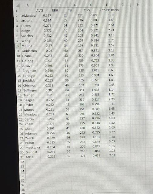
please hep using R program

Use R to construct scatterplots for all pairs of attributes. (As there are five attributes, you will create a total of ten scatterplots.) Among this set of plots, choose the one that best displays linear correlation, and paste only that scatterplot below. In a sentence or two, justify your attribute pair selection.

For the attribute pair you selected in Problem 1, construct the linear model using the lm command, provide a summary of values using the summary command, and draw the regression line on top of your scatterplot using the abline command. Give all R code and output, including the new plot containing both the points and the regression line, below.Save this file in your working directory, and assign it to batters in R.,

Suppose now that you wish to introduce a third attribute, and provide a multiple linear regression model that pairs the new attribute with the two attributes for which you provided a simple linear regression model. Which attribute will you choose as your third, and why? Justify your choice in a sentence or two. Use the lm and summary commands to construct the new linear model, and to list a summary of values. Provide all R code and output below.

D F G H 61 55 64 46 47 40 34 60 53 62 61 A B 1 AVG EBH 2 LeMahieu 0.327 3. Urshela 0.314 4 Torres 0.278 5 Judge 0.272 6 Sanchez 0.232 7 Wong 0.285 8 Molina 0.27 9 Goldschm 0.26 10 Ozuna 0.243 11 Delong 0.233 12 Altuve 0.298 13 Bregman 0.296 14 Springer 0.292 15 Reddick 0.275 16. Chirinos 0.238 17 Bellinger 0.305 18 Turner 0.29 19 Seager 0.272 20 Taylor 0.262 21 Muncy 0.251 22 Meadows 0.291 23 Garcia 0.282 24 Phan 0.273 25 Chi 0.261 26 Adames 0.254 27 Yelich 0.329 28 Braun 0.285 29 Moustaka 0.254 30 Grandal 0.246 31 Arcia 0.223 32 33 80 62 36 40 84 OPS K to BB Ratio 312 0.893 1.95 236 0.889 3.48 292 0.821 2.64 204 0.921 2.21 208 0.841 3.13 202 0.784 1.76 167 0.711 2.52 284 0.821 2.13 230 0.804 1.84 259 0.762 2.39 275 0.903 1.98 328 1.015 0.59 283 0.974 1.69 205 0.728 1.83 162 0.791 2.45 351 1.035 1.14 244 0.881 1.72 236 0.817 2.23 169 0.794 3.11 251 0.889 1.65 296 0.922 2.43 227 0.796 4.03 255 0.818 1.52 188 0.822 1.69 22 0.735 3.32 328 1.101 1.48 232 0.849 3.09 270 0.845 1.85 240 0.848 1.28 173 0.633 2.53 51 64 45 58 69 47 56 41 46 76 55 66 56 32 34 35 36 37 38 D F G H 61 55 64 46 47 40 34 60 53 62 61 A B 1 AVG EBH 2 LeMahieu 0.327 3. Urshela 0.314 4 Torres 0.278 5 Judge 0.272 6 Sanchez 0.232 7 Wong 0.285 8 Molina 0.27 9 Goldschm 0.26 10 Ozuna 0.243 11 Delong 0.233 12 Altuve 0.298 13 Bregman 0.296 14 Springer 0.292 15 Reddick 0.275 16. Chirinos 0.238 17 Bellinger 0.305 18 Turner 0.29 19 Seager 0.272 20 Taylor 0.262 21 Muncy 0.251 22 Meadows 0.291 23 Garcia 0.282 24 Phan 0.273 25 Chi 0.261 26 Adames 0.254 27 Yelich 0.329 28 Braun 0.285 29 Moustaka 0.254 30 Grandal 0.246 31 Arcia 0.223 32 33 80 62 36 40 84 OPS K to BB Ratio 312 0.893 1.95 236 0.889 3.48 292 0.821 2.64 204 0.921 2.21 208 0.841 3.13 202 0.784 1.76 167 0.711 2.52 284 0.821 2.13 230 0.804 1.84 259 0.762 2.39 275 0.903 1.98 328 1.015 0.59 283 0.974 1.69 205 0.728 1.83 162 0.791 2.45 351 1.035 1.14 244 0.881 1.72 236 0.817 2.23 169 0.794 3.11 251 0.889 1.65 296 0.922 2.43 227 0.796 4.03 255 0.818 1.52 188 0.822 1.69 22 0.735 3.32 328 1.101 1.48 232 0.849 3.09 270 0.845 1.85 240 0.848 1.28 173 0.633 2.53 51 64 45 58 69 47 56 41 46 76 55 66 56 32 34 35 36 37 38