Please only answer question 3, question 2 has theory that you might need to answer question 3 that is why I have attached it too. For question 3, please provide complete solution, show full calculations, explanations and proofs.

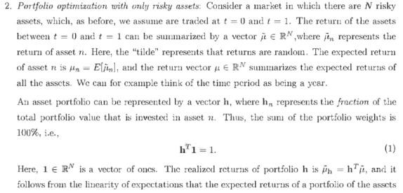
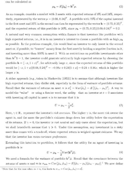
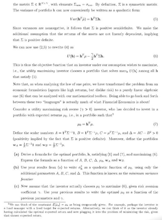
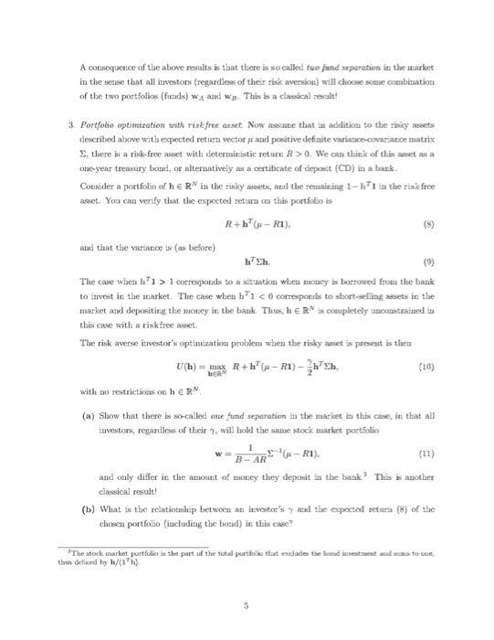
2. Portfolio optimization with only risky assets: Consider a market in which there are N risky assets, which, as before, we assume are traded at t = 0 and t = 1. The return of the assets between t = 0 and t = 1 can be summarized by a vector i E RN where in represents the return of asset n. Here, the "tilde" represents that returns are random. The expected return of asset it is An = Elind, and the return vector HE RN summarizes the expected returns of all the assets. We can for example think of the time period as being a year. An asset portfolio can be represented by a vector h, where he represents the fraction of the total portfolio value that is invested in asset . Thus, the sum of the portfolio weights is 100%. i.e., h"1=1. (1) Here, 1 E R is a vector of ones. The realized returns of portfolio h is in = hit, and it follows from the linearity of expectations that the expected returns of a portfolio of the assets can be calculated as El = h' (2) As an example, consider a market with 2 assets with expected returns of 8% and 24%, respec tively, represented by the vector de = (0.08, 0.24) A portfolio with 75% of the capital invested in the first asset and 25% in the second can then be represented by the vector h = (0.75,0.25) and the expected return of this portfolio is 20%, since it = (0.75, 0.25)(0.08.0.24)" = 0.2 A natural and very common assumption within finance is that investors like portfolios with high expected returns, i.e., it is in an investor's interest to choose a portfolio with a high as possible. In the previous example, this would lead an investor to only invest in the second assct or if possible to borrow" moncy from the first asset by holding a negative fraction in it, and investing more than 100% in asset 2 With no restrictions on portfolio investments otser thanh' 1 - 1, the investor could generate arbitrarily high expected returres by choosing the portfolio h = (-1, 1+x)". for arbitrarily large I, since the expected returns of this portfolio would be (-1,1 + x)(0.08,0.24) * = -0,082 +0.24(1 + 2) = 0.24 +0.16r, which is higher the larger ris. A richer approach (e.g., taken in Markowitz (1952)) is to assume that although izvestors like high expected returns they dislike risk, especially in the form of varianoe of portfolio returns. Recall that the variance of returns classet niso - Var() - (An - Hu)?). A way to model the value or tising a fancier word, the utility that an investor at t=0 associates with investing all capital in asset n is to assume that it is (3) Here, 7 R. represent the investor's risk version. The higher is, the more risk averse the agent is, and the more the portfolio's riskiness drags down her utility below the expectation of its retures. If y = 0, the investor is risk neutral and only cares about the expectation, but we shall licnceforth assume that y > 0. Under this assumption, any investment in a risky assct this comes with a tradeoff, were expected return is weighed against riskuess. We say that the investor has mean-variance preferences Extending this intuition to portfolios, it follows that the utility for an agent of investing in portfolio his U = "-Var(h"). We need a formula for the variance of portfolio h". Rocall that the covariance between the returns of assets n and mis onm = Covljite n) = E|--H)].? We now define Note that for the case wher, this leads to it. Col.) the matrix SERVx, with clements Com By definition, is a symmetric matrix The variance of portfolio h can now conveniently be written as a quadratic form: Var(h") = heh. (5) Since variances are nonnegative, it follows that is positive senidetinite. We make the additional assumption that the returns of the assets are not linearly dependent, implying that is positive definite. We can now use (2,5) to rewrite (4) as (6) This is thus the objective function that an investor under our assumption wishes to maximize, ie, the utility maximizing investor chooses a portfolio that solves max. (h) among all h that satisfy (1) Note that, as when analyzing the law of one price, we have transformed the problem from an economic forumlation (agents like light returns, but dislike risk) to a purely linear algebraic oue (6) that can be analyzed with our mathematical toolbox. Being able to go back and forth between these two "languages" is actually much of what Financial Economics is about! Consider a utility maximizing risk averse (> 0) investor, who has decided to invest in a portfolio with expected returns tule, in a portfolio such that? (7) Define the scalar mmbers A = 175-1, B=175+ C = "--, and A = AC-B2 > 0 (positivity implied by the fact that is positive definite). Moreover, vefine the portfolios WA = 481 and we = . (a) Derive a formula for the optimal portfolio, h, satisfying (1) and (7), and maximizing (6) Express the formula as a function of A, B, C, A, HO WA and we (b) Use your results from (a) to write of as a quadratic function of Housing only the additional parameters A, B, C, and A This function is known as the minimum wariance frontier (c) Now assume that the investor actually chooses to to watimize (6), given risk aversion coefficient 7. Use your previous results to write the optimal Ho as a function of thic previous parameters and * We can think of the constraint EwHo as being coasty given For example, perhaps the investotis a fund nuper with a fixed target for expected returns Alternatively, we can think of it as the investur already having calculated the optimal expected return and now plugging it into the problem of minimizing the risk given that chosen expected retum. A consequence of the above results is that there is so called two jund separation in the market in the sense that all investors (regardless of their risk aversion) will choose some combination of the two portfolios (funds) wAand wg. This is a classical result 3 Portfolio optimization with risk-free asset Now assue that an addition to the riskynsets described above with expected return vector je nad positive definite variatico.cariance matrix Ethere it a risk-froe nect with deterministic retur R > 0. We can think of this aset as a one-year trentury brand, or alternatively as a certificate of deposit (CD) in a bank Consider a portfolio of her in the risky anets, and the remaining 1-b1 in the risk free asset. You can verify that the expected return co this portfolio is R+"-RI). (5) and that the variance is (as before) (9) The case wlicni b'1 > 1 corresponds to a situation when money is borrowed from the bank to invest in the market. The case when t'i 0. Under this assumption, any investment in a risky assct this comes with a tradeoff, were expected return is weighed against riskuess. We say that the investor has mean-variance preferences Extending this intuition to portfolios, it follows that the utility for an agent of investing in portfolio his U = "-Var(h"). We need a formula for the variance of portfolio h". Rocall that the covariance between the returns of assets n and mis onm = Covljite n) = E|--H)].? We now define Note that for the case wher, this leads to it. Col.) the matrix SERVx, with clements Com By definition, is a symmetric matrix The variance of portfolio h can now conveniently be written as a quadratic form: Var(h") = heh. (5) Since variances are nonnegative, it follows that is positive senidetinite. We make the additional assumption that the returns of the assets are not linearly dependent, implying that is positive definite. We can now use (2,5) to rewrite (4) as (6) This is thus the objective function that an investor under our assumption wishes to maximize, ie, the utility maximizing investor chooses a portfolio that solves max. (h) among all h that satisfy (1) Note that, as when analyzing the law of one price, we have transformed the problem from an economic forumlation (agents like light returns, but dislike risk) to a purely linear algebraic oue (6) that can be analyzed with our mathematical toolbox. Being able to go back and forth between these two "languages" is actually much of what Financial Economics is about! Consider a utility maximizing risk averse (> 0) investor, who has decided to invest in a portfolio with expected returns tule, in a portfolio such that? (7) Define the scalar mmbers A = 175-1, B=175+ C = "--, and A = AC-B2 > 0 (positivity implied by the fact that is positive definite). Moreover, vefine the portfolios WA = 481 and we = . (a) Derive a formula for the optimal portfolio, h, satisfying (1) and (7), and maximizing (6) Express the formula as a function of A, B, C, A, HO WA and we (b) Use your results from (a) to write of as a quadratic function of Housing only the additional parameters A, B, C, and A This function is known as the minimum wariance frontier (c) Now assume that the investor actually chooses to to watimize (6), given risk aversion coefficient 7. Use your previous results to write the optimal Ho as a function of thic previous parameters and * We can think of the constraint EwHo as being coasty given For example, perhaps the investotis a fund nuper with a fixed target for expected returns Alternatively, we can think of it as the investur already having calculated the optimal expected return and now plugging it into the problem of minimizing the risk given that chosen expected retum. A consequence of the above results is that there is so called two jund separation in the market in the sense that all investors (regardless of their risk aversion) will choose some combination of the two portfolios (funds) wAand wg. This is a classical result 3 Portfolio optimization with risk-free asset Now assue that an addition to the riskynsets described above with expected return vector je nad positive definite variatico.cariance matrix Ethere it a risk-froe nect with deterministic retur R > 0. We can think of this aset as a one-year trentury brand, or alternatively as a certificate of deposit (CD) in a bank Consider a portfolio of her in the risky anets, and the remaining 1-b1 in the risk free asset. You can verify that the expected return co this portfolio is R+"-RI). (5) and that the variance is (as before) (9) The case wlicni b'1 > 1 corresponds to a situation when money is borrowed from the bank to invest in the market. The case when t'i