Please show matlab code
-------------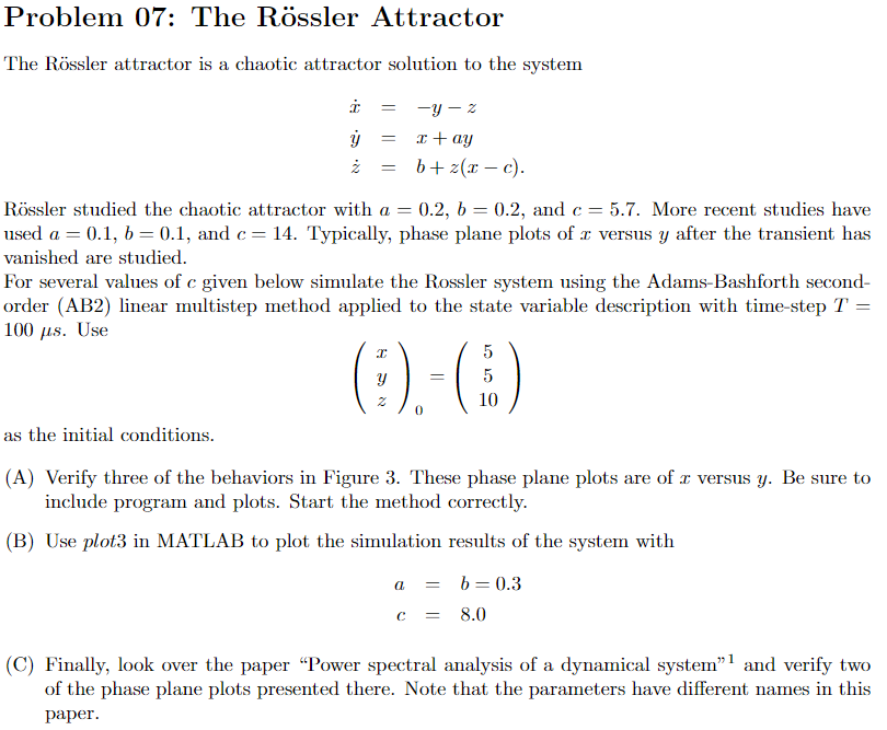
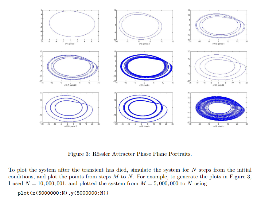
Problem 07: The Rssler Attractor The Rssler attractor is a chaotic attractor solution to the system . y = = = -y - 2 1+ay b+ (1 -c). Rssler studied the chaotic attractor with a = 0.2, b = 0.2, and c=5.7. More recent studies have used a = 0.1, b = 0.1, and c= 14. Typically, phase plane plots of 3 versus y after the transient has vanished are studied. For several values of c given below simulate the Rossler system using the Adams-Bashforth second- order (AB2) linear multistep method applied to the state variable description with time-step T = 100 us. Use =15 as the initial conditions. (A) Verify three of the behaviors in Figure 3. These phase plane plots are of 3 versus y. Be sure to include program and plots. Start the method correctly. (B) Use plot3 in MATLAB to plot the simulation results of the system with a C = = b = 0.3 8.0 (C) Finally, look over the paper "Power spectral analysis of a dynamical system" and verify two of the phase plane plots presented there. Note that the parameters have different names in this paper. 00 Figure 3: Rssler Attracter Phase Plane Portraits. To plot the system after the transient has died, simulate the system for N steps from the initial conditions, and plot the points from steps M to N. For example, to generate the plots in Figure 3, I used N = 10,000,001, and plotted the system from M = 5,000,000 to N using plot (x (5000000:N) , (5000000:N)) Problem 07: The Rssler Attractor The Rssler attractor is a chaotic attractor solution to the system . y = = = -y - 2 1+ay b+ (1 -c). Rssler studied the chaotic attractor with a = 0.2, b = 0.2, and c=5.7. More recent studies have used a = 0.1, b = 0.1, and c= 14. Typically, phase plane plots of 3 versus y after the transient has vanished are studied. For several values of c given below simulate the Rossler system using the Adams-Bashforth second- order (AB2) linear multistep method applied to the state variable description with time-step T = 100 us. Use =15 as the initial conditions. (A) Verify three of the behaviors in Figure 3. These phase plane plots are of 3 versus y. Be sure to include program and plots. Start the method correctly. (B) Use plot3 in MATLAB to plot the simulation results of the system with a C = = b = 0.3 8.0 (C) Finally, look over the paper "Power spectral analysis of a dynamical system" and verify two of the phase plane plots presented there. Note that the parameters have different names in this paper. 00 Figure 3: Rssler Attracter Phase Plane Portraits. To plot the system after the transient has died, simulate the system for N steps from the initial conditions, and plot the points from steps M to N. For example, to generate the plots in Figure 3, I used N = 10,000,001, and plotted the system from M = 5,000,000 to N using plot (x (5000000:N) , (5000000:N))