Answered step by step
Verified Expert Solution
Link Copied!

Question

1 Approved Answer

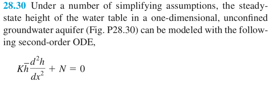
Please use MATLAB. Thank you. 28.30 Under a number of simplifying assumptions, the steady state height of the water table in a one-dimensional, unconfined groundwater

Please use MATLAB. Thank you.

image text in transcribedimage text in transcribed

image text in transcribed

image text in transcribed

28.30 Under a number of simplifying assumptions, the steady state height of the water table in a one-dimensional, unconfined groundwater aquifer (Fig. P28.30) can be modeled with the follow- ing second-order ODE dx dy cy+dxy dt where K -the carrying capacity. Use the same parameter values and initial conditions as in Sec. 28.2 to integrate these equations from t -0 to 100 using ode45. (a) Employ a very large value of K 10 to validate that you ob- tain the same results as in Sec. 28.2. Solution. Use the following parameter values for the predator-prey simulation: a-1.2 b = 0.6, C 0.8, and d = 0.3. Employ initial conditions of x = 2 and y = 1 and inte- grate from t = 0 to 30, we will use the fourth-order RK method with double precision to obtain solutions. Solve with the linear shooting method. (In Lecture 14 we already solved this problem using the finite difference method). Submit a plot of h(x) along with your code. Because the ODE is linear, you only need to evaluate two "shots" to find the correct initial conditions. Report the slopes and resulting right-side boundary values that you find. Use any ODE solution technique that you prefer (RK4 or built-in ode45). 28.30 Under a number of simplifying assumptions, the steady state height of the water table in a one-dimensional, unconfined groundwater aquifer (Fig. P28.30) can be modeled with the follow- ing second-order ODE dx dy cy+dxy dt where K -the carrying capacity. Use the same parameter values and initial conditions as in Sec. 28.2 to integrate these equations from t -0 to 100 using ode45. (a) Employ a very large value of K 10 to validate that you ob- tain the same results as in Sec. 28.2. Solution. Use the following parameter values for the predator-prey simulation: a-1.2 b = 0.6, C 0.8, and d = 0.3. Employ initial conditions of x = 2 and y = 1 and inte- grate from t = 0 to 30, we will use the fourth-order RK method with double precision to obtain solutions. Solve with the linear shooting method. (In Lecture 14 we already solved this problem using the finite difference method). Submit a plot of h(x) along with your code. Because the ODE is linear, you only need to evaluate two "shots" to find the correct initial conditions. Report the slopes and resulting right-side boundary values that you find. Use any ODE solution technique that you prefer (RK4 or built-in ode45)

Step by Step Solution

There are 3 Steps involved in it

Step: 1

blur-text-image

Get Instant Access to Expert-Tailored Solutions

See step-by-step solutions with expert insights and AI powered tools for academic success

Step: 2

blur-text-image

Step: 3

blur-text-image

Ace Your Homework with AI

Get the answers you need in no time with our AI-driven, step-by-step assistance

Get Started

Students also viewed these Databases questions