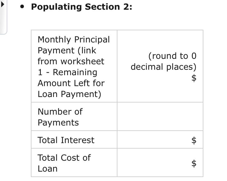
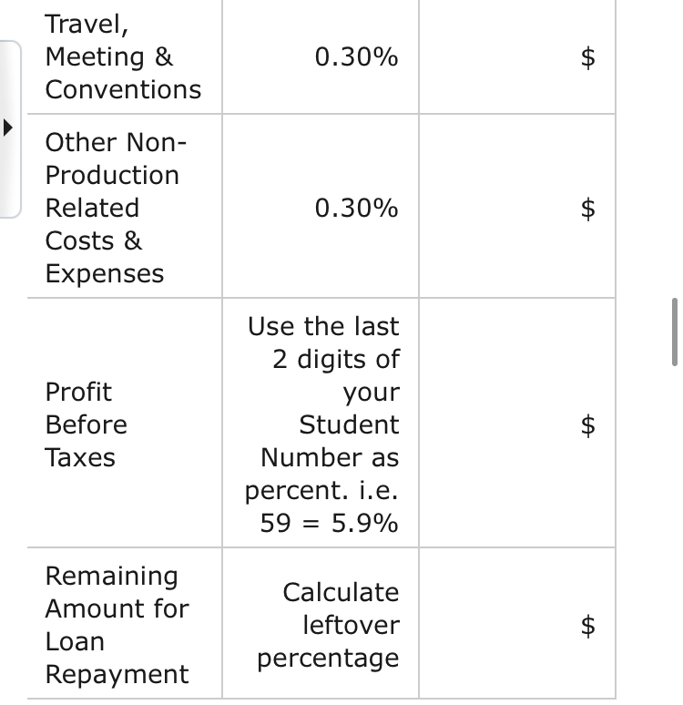
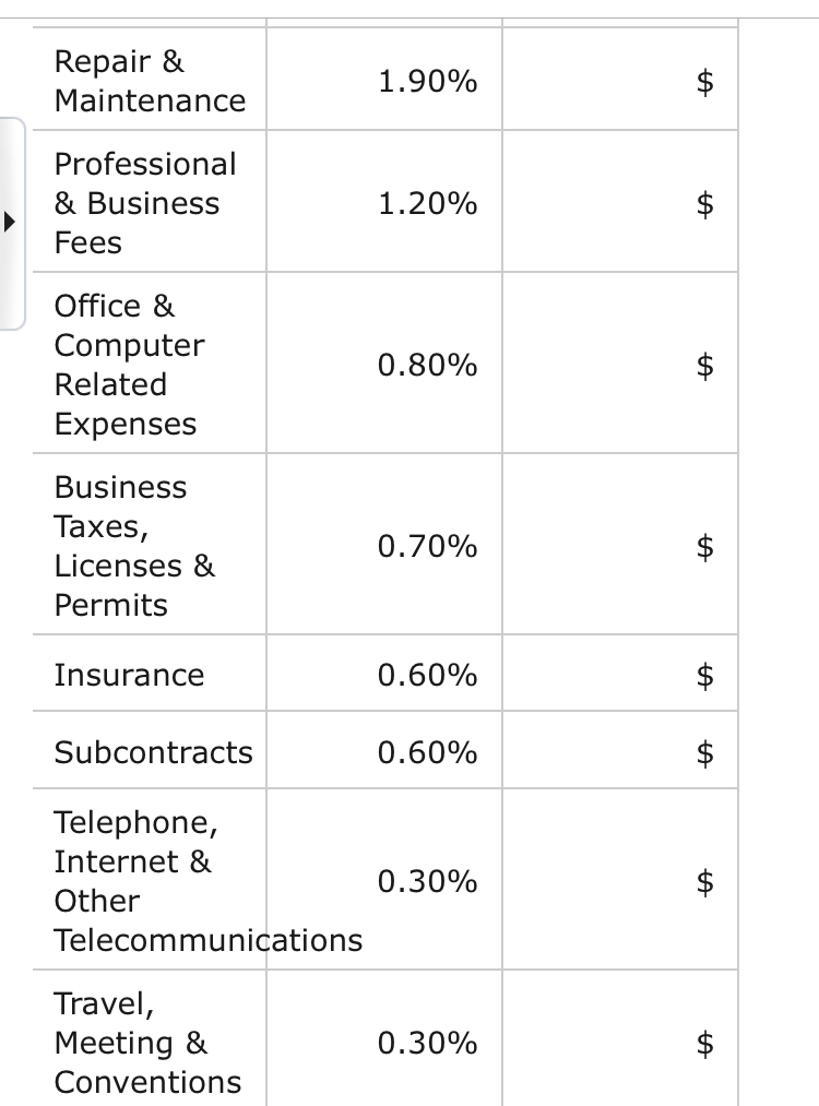
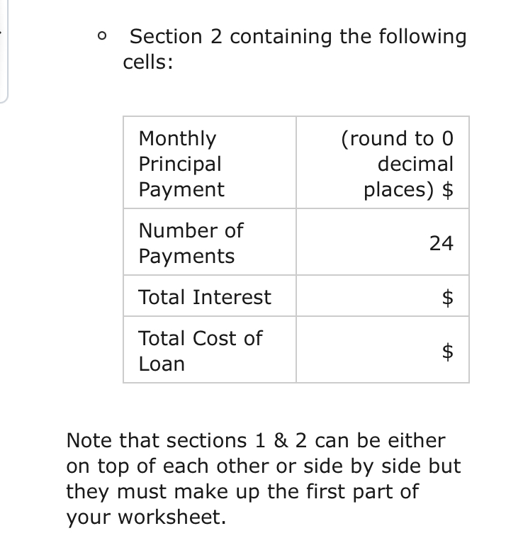
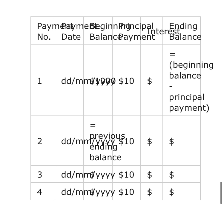
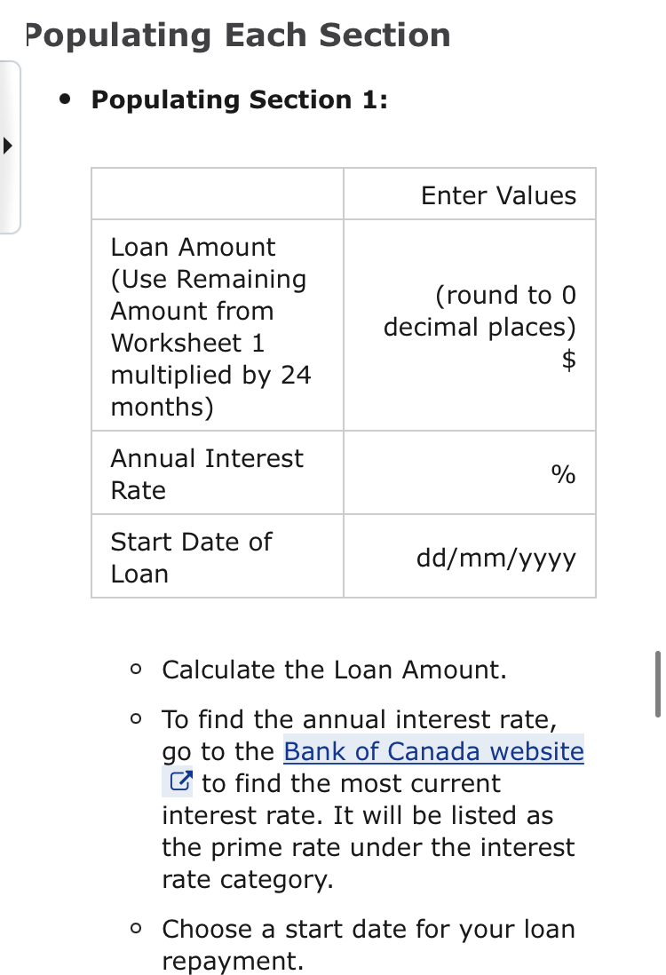
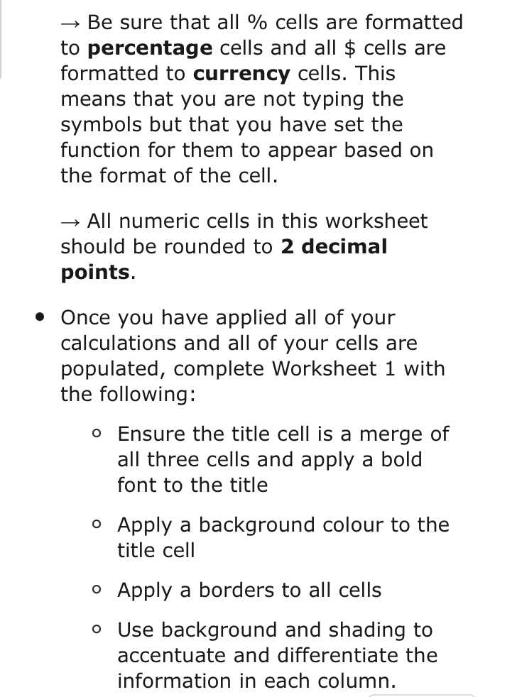
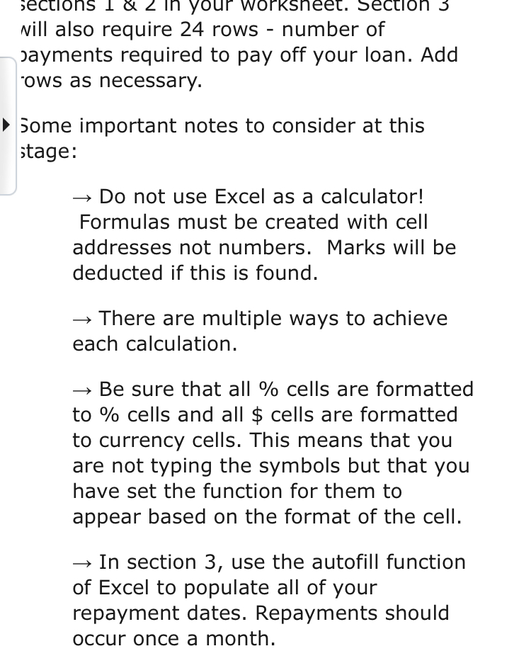
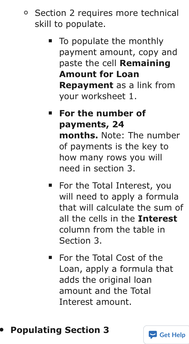
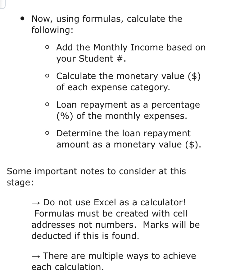
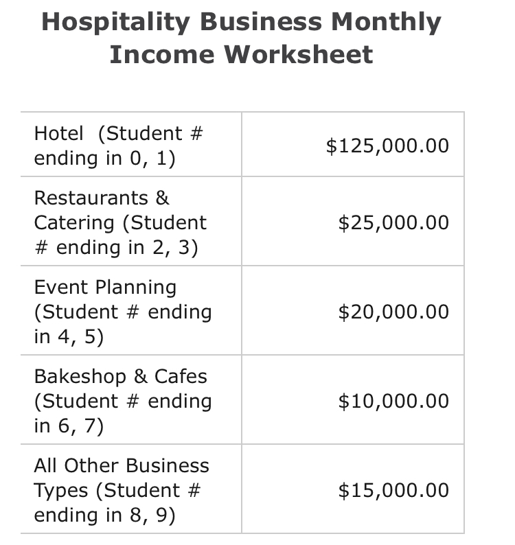
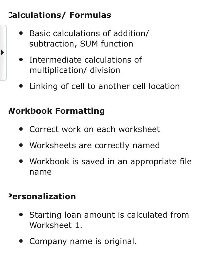
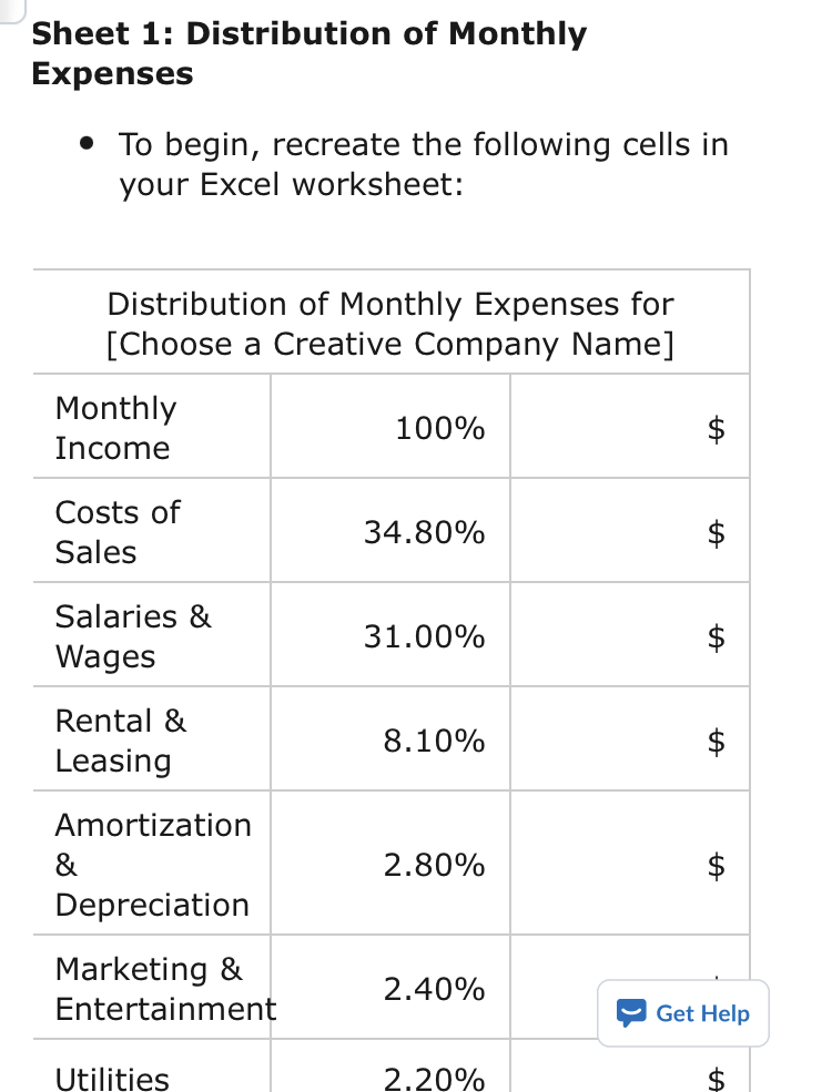
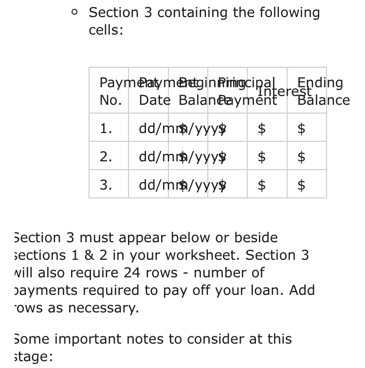
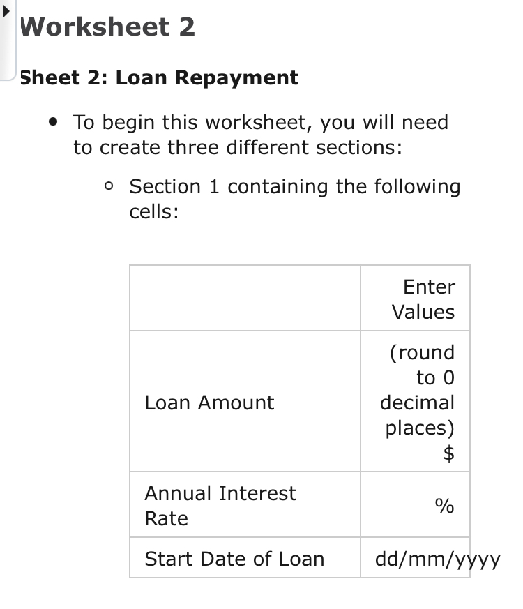
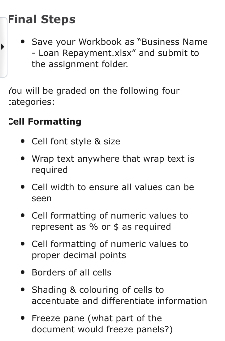
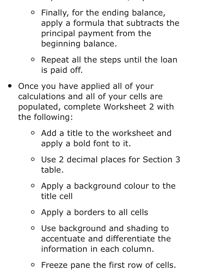
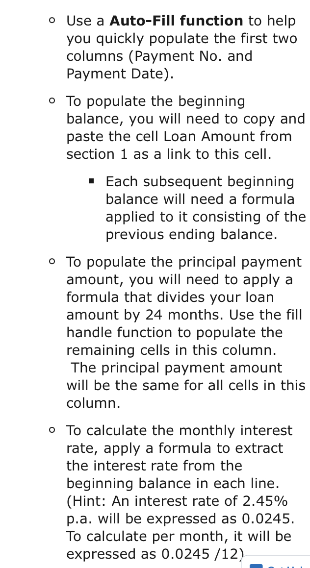
. Populating Section 2: Monthly Principal Payment (link from worksheet (round to 0 1 - Remaining decimal places) LA Amount Left for Loan Payment) Number of Payments Total Interest $ Total Cost of $ LoanTravel, Meeting & 0.30% $ Conventions Other Non- Production Related 0.30% $ Costs & Expenses Use the last 2 digits of Profit your Before Student $ Taxes Number as percent. i.e. 59 = 5.9% Remaining Calculate Amount for leftover Loan Repayment percentageRepair & 1.90% Maintenance Professional & Business 1.20% $ Fees Office & Computer 0.80% Related Expenses Business Taxes, 0.70% Licenses & Permits Insurance 0.60% Subcontracts 0.60% $ Telephone, Internet & 0.30% $ Other Telecommunications Travel, Meeting & 0.30% Conventions0 Section 2 containing the following cells: Monthly (round to 0 Principal decimal Payment places) $ Number of 24 Payments Total Interest $ Total Cost of $ Loan Note that sections 1 & 2 can be either on top of each other or side by side but they must make up the rst part of your worksheet. PaymeatymeBeginnPrincipal Ending Interest No. Date Balanceayment Balance (beginning dd/mm$1909 $10 balance 1 $ principal payment) previous, 2 dd/mm ending $10 $ $ balance 3 dd/mm$/yyyy $10 $ 4 dd/mm$yyyy $10Populating Each Section I Populating Section 1: Enter Values Loan Amount (Use Remaining (round to 0 Amount from decimal laces) Worksheet 1 p $ multiplied by 24 months) Annual Interest 0/ Rate 0 Start Date of dd/mm/YWY Loan 0 Calculate the Loan Amount. 0 To nd the annual interest rate, go to the Bank of Canada website 13' to find the most current interest rate. It will be listed as the prime rate under the interest rate category. 0 Choose a start date for your loan repayment. } Be sure that all % cells are formatted to percentage cells and all $ cells are formatted to currency cells. This means that you are not typing the symbols but that you have set the function for them to appear based on the format of the cell. ;. All numeric cells in this worksheet should be rounded to 2 decimal points. Once you have applied all of your calculations and all of your cells are populated, complete Worksheet 1 with the following: 0 Ensure the title cell is a merge of all three cells and apply a bold font to the title 0 Apply a background colour to the title cell 0 Apply a borders to all cells 0 Use background and shading to accentuate and differentiate the information in each column. sections 1 o a in your worKsneet. bECtlon 5 Will also require 24 rows number of Jayments required to pay off your loan. Add "ows as necessary. Some important notes to consider at this wage: _} Do not use Excel as a calculator! Formulas must be created with cell addresses not numbers. Marks will be deducted if this is found. } There are multiple ways to achieve each calculation. _} Be sure that all \"/0 cells are formatted to % cells and all $ cells are formatted to currency cells. This means that you are not typing the symbols but that you have set the function for them to appear based on the format of the cell. _} In section 3, use the autofil] function of Excel to populate all of your repayment dates. Repayments should occur once a month. 0 Section 2 requires more technical skill to populate. I To populate the monthly payment amount, copy and paste the cell Remaining Amount for Loan Repayment as a link from your worksheet 1. I For the number of payments, 24 months. Note: The number of payments is the key to how many rows you will need in section 3. I For the Total Interest, you will need to apply a formula that will calculate the sum of all the cells in the Interest column from the table in Section 3. I For the Total Cost of the Loan, apply a formula that adds the original loan amount and the Total Interest amount. .- Populating Section 3 g GetHelp I Now, using formulas, calculate the following: 0 Add the Monthly Income based on your Student #. 0 Calculate the monetary value ($) of each expense category. 0 Loan repayment as a percentage (\"/o) of the monthly expenses. 0 Determine the loan repayment amount as a monetary value ($). Some important notes to consider at this stage: } Do not use Excel as a calculator! Formulas must be created with cell addresses not numbers. Marks will be deducted if this is found. } There are multiple ways to achieve each calculation. Hospitality Business Monthly Income Worksheet Hotel (Student # ending in 0, 1) $125,000.00 Restaurants & Catering (Student $25,000.00 # ending in 2, 3) Event Planning (Student # ending $20,000.00 in 4, 5) Bakeshop & Cafes (Student # ending $10,000.00 in 6, 7) All Other Business Types (Student # $15,000.00 ending in 8, 9)Calculations/ Formulas . Basic calculations of addition/ subtraction, SUM function . Intermediate calculations of multiplication/ division . Linking of cell to another cell location Workbook Formatting . Correct work on each worksheet . Worksheets are correctly named . Workbook is saved in an appropriate file name Personalization . Starting loan amount is calculated from Worksheet 1. . Company name is original.Sheet 1: Distribution of Monthly Expenses - To begin, recreate the following cells in your Excel worksheet: Distribution of Monthly Expenses for [Choose a Creative Company Name] Monthly Income Costs of Sales Salaries & Wages Rental & Leasing Amortization & Depreciation Marketing & Entertainment Utilities 100% 34.80% 31.00% 8.10% 2.80% 2.40% 2.20% a Get Help o Section 3 containing the following cells: Paymeatymedgin RimigciPatending No. Date Balandayment Balance 1. dd/mrs/yyy$ 2. dd/mrs/yyy$ 3. dd/mm/yyy$ LA Section 3 must appear below or beside sections 1 & 2 in your worksheet. Section 3 will also require 24 rows - number of payments required to pay off your loan. Add ows as necessary. Some important notes to consider at this stage:' Worksheet 2 Sheet 2: Loan Repayment I To begin this worksheet, you will need to create three different sections: 0 Section 1 containing the following cells: Enter Values (round to 0 Loan Amount decimal places) $ Annual Interest 0 Rate A] Start Date of Loan dd/mm/yyyy Final Steps I Save your Workbook as \"Business Name Loan Repaymentxlsx" and submit to the assignment folder. r'ou will be graded on the following four :ategories: :ell Formatting I Cell font style & size I Wrap text anywhere that wrap text is required I Cell width to ensure all values can be seen I Cell formatting of numeric values to represent as 0/0 or $ as required I Cell formatting of numeric values to proper decimal points I Borders of all cells I Shading & colouring of cells to accentuate and differentiate information I Freeze pane (what part of the document would freeze panels?) 0 Finally, for the ending balance, apply a formula that subtracts the principal payment from the beginning balance. 0 Repeat all the steps until the loan is paid off. I Once you have applied all of your calculations and all of your cells are populated, complete Worksheet 2 with the following: 0 Add a title to the worksheet and apply a bold font to it. 0 Use 2 decimal places for Section 3 table. 0 Apply a background colour to the title cell 0 Apply a borders to all cells 0 Use background and shading to accentuate and differentiate the information in each column. 0 Freeze pane the first row of cells. 0 Use a Auto-Fill function to help you quickly populate the first two columns (Payment No. and Payment Date). 0 To populate the beginning balance, you will need to copy and paste the cell Loan Amount from section 1 as a link to this cell. I Each subsequent beginning balance will need a formula applied to it consisting of the previous ending balance. 0 To populate the principal payment amount, you will need to apply a formula that divides your loan amount by 24 months. Use the fill handle function to populate the remaining cells in this column. The principal payment amount will be the same for all cells in this cmumn. 0 To calculate the monthly interest rate, apply a formula to extract the interest rate from the beginning balance in each line. (Hint: An interest rate of 2.45% pa will be expressed as 0.0245. To calculate per month, it will be expressed as 0.0245 /12) Instructions Follow the steps below to complete the D . assignment: Workbook: Begin by creating a new workbook. In the workbook you will want to have 2 worksheets. Name your worksheets as follows: I Sheet 1: Monthly Expenses I Sheet 2: Loan Repayment Plan
